3 A Geometric Morphometric and Machine Learning Approach to Regional Projectile Point Analysis in the Southwest United States
3.1 Introduction
Projectile points, and stone tools in general, are rarely the subject of regional-scale studies in the post-archaic era of the U.S. Southwest (for some exceptions see Cameron 2001; Hoffman 1997; Justice 2002a; Loendorf 2010; Paige 2022; Ryan 2017; Sedig 2014; Sliva 1999, 2006; Whittaker and Bryce 2017). One problem with a regional analysis for projectile points is that numerous type names and schemas have been devised, often ad hoc, across the Southwest. This complicates comparisons, as the number of type names likely exceeds the number of distinct styles (Sliva 2006, p. 37). A relatively new method for projectile point analysis is drawn from the field of geometric morphometrics (GMM). GMM enables us to measure shape differences more objectively, without depending on traditional classification systems. While GMM can help identify differences in morphology, the rapid development of machine learning means we can automate projectile point analyses once an appropriate procedure and training dataset has been created. Of course the problem of harmonizing or even creating regional projectile point typologies is not limited to the Southwest U.S. This article is not meant to create a new typology for general use. Rather, it is a case study on conducting regional-scale analyses of projectile points using GMM for the purposes of examining regional scale interaction.
Projectile point styles are often associated with social identity (Mason 1894, p. 655; Waguespack et al. 2009, p. 787; Whittaker 1994, pp. 260–268). This is not always the case, though there is evidence there is some association between projectile point types and known cultural groups in the Southwest. Functional differences in projectile point types cannot, however, be ignored as a contributing factor to stylistic differences. Projectile point styles in the Southwest, particularly the type of hafting, are affected by their intended purpose. Hunting and warfare have different requirements for optimal projectile point performance which affects point morphology (Loendorf et al. 2015).
Ecological variation can also affect morphology. A recent study of Central African hunter-gatherers found subsistence tools, including projectiles, were less frequently exchanged than musical instruments and more adapted to local ecologies (Padilla-Iglesias et al. 2024). In the Southwest there are a limited number of large game animals that inhabit most of the region, thus large game animals are not expected to form local ecological niches. Large game animals are noted because stone points were typically not used for small game (Ellis 1997; Loendorf et al. 2015; Waguespack et al. 2009).
Besides ecological reasons for morphology differences, resharpening and repurposing can affect the typology of projectile points (e.g., Bamforth 1991; Gardner and Verrey 1979; Hoffman 1985; Larick 1985). Fortunately, experiments with the type of small arrow points considered in this study demonstrate this is unlikely to be a significant factor (Loendorf et al. 2019). Loendorf and colleagues found through experimental research that most small arrow points cannot be reworked when damaged while firing. Also, because the points may have been more work to reattach to the arrow than to make another, the bases are unlikely to have been commonly reworked. Azevedo and colleagues (2014) studied the morphology of points after tool modification and found that the original shape was still the primary factor in the overall variation. They also note that arrow point tips are most affected by resharpening, echoing the work of Loendorf and colleagues. Because the base of the point is less likely to be affected by reworking in general, and the base is the primary discriminant between types in the Southwest (Justice 2002a; Sliva 1997, 2006), resharpening is not likely to be an important factor in this analysis.
Ethnographic and archaeological sources in the Southwest document the use or association of projectile points with various social and symbolic functions (Bayman 2007, pp. 78–79; Beaglehole 1936; Cushing 1883; Dittert 1959; Fewkes 1898; Justice 2002a, pp. 309–310; Kaldahl 2000; Kamp et al. 2016; Parsons 1932, 1939; Russell 1908; Sedig 2014; Simpson 1953; J. Stevenson 1884; M. C. Stevenson 1894, 1903; Whittaker and Kamp 2016). These factors suggest that social differences play a substantial role in projectile point style, and thus, there is some association with recognized archaeological cultures and projectile point styles. I presume that similarities in projectile point styles represent interaction, however, it is also possible that identical point styles can independently be invented in multiple areas (i.e., convergence). I assume interaction/diffusion as the default explanation because all of the areas in my study area are known to have interacted and exchanged goods.
The primary goal of this study is to examine and develop heuristics for efficiently examining regional variation in projectile points using GMM methods and machine learning. Besides difficulties with typologies, analyzing sufficient numbers of projectile points for a suitable regional analysis is an expensive process at least in time and typically also in resources. The use of GMM and machine learning can help to automate the analysis and reduce the time and resources needed to conduct a regional analysis. This study will examine the utility of these methods for a regional analysis of projectile points.
Goals:
- Discrimination – Determine whether GMM can distinguish projectile point types.
- Method Selection – Identify optimal GMM approaches.
- Automation – Improve reproducibility and efficiency using machine learning.
- Regional Analysis – Explore projectile point distributions across the Southwest.
To address these objectives, this case study focuses on a large region of the central U.S. Southwest during the late pre-Hispanic period between AD 1100 and 1500. This period and location present an opportunity to examine projectile point variation across several archaeological culture areas and during a time of marked social change. By analyzing a large collection of projectile points from this region, this study provides a methodological framework for conducting regional-scale analyses of projectile points.
3.1.1 Study Region: Central U.S. Southwest, AD 1100–1500.
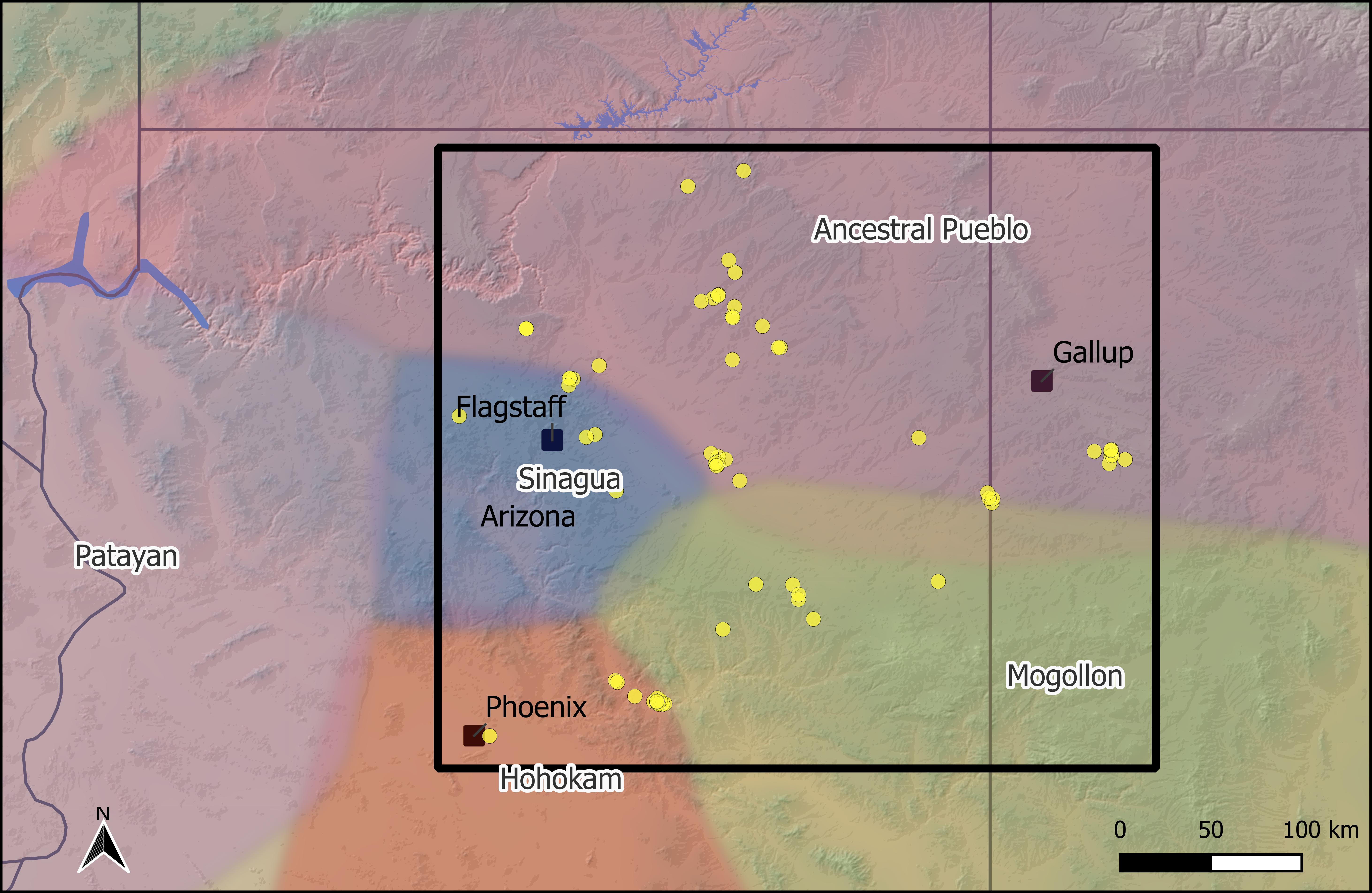
The project area (Figure 3.1) includes a large portion of northern Arizona and northwest New Mexico extending from the Tonto Basin below the Mogollon Rim to areas near Monument Valley on the north and the Flagstaff area in the west to the Zuni Mountains in the east. It also includes the site of S’edav Va’aki (formerly known as Pueblo Grande), from the Phoenix Basin, which was added for an additional comparative site. This large area encompasses a diverse landscape across which archaeologists have defined multiple archaeological culture areas (Ancestral Pueblo, Mogollon, Sinagua, Hohokam) and regional traditions (Kayenta, Cibola, and others). This extent includes much of the contemporary and traditional lands of both Hopi and Zuni Pueblos. Relationships between archaeological culture area designations and groups of people with shared identities are obviously complex (Duff 2002; M. A. Peeples 2018), but the scope of the region defined here is certainly large enough to capture cultural variation that spans many distinct social boundaries and identities.
This area and time period provide an excellent context for exploring variation in projectile point design and distribution. The study’s geographical and cultural scope allows for examining potential boundaries in stylistic distributions across distinct regions and culture areas. Interaction was common between these regions (e.g., E. Charles Adams et al. 1993; Bernardini 2005; Bischoff 2023a; J. J. Clark 2001; Duff 2000, 2004; Gauthier 2021; B. J. Mills et al. 2013, 2015; M. Peeples et al. 2021; M. A. Peeples 2018; M. A. Peeples and Haas 2013; Stark et al. 1998). Between AD 1100 and 1200, populations grew throughout the study region (Bernardini et al. 2021; Dean 2010; Hill et al. 2004), while major societal changes occurred after the end of the Chacoan regional system around the middle of the century (Cameron and Duff 2008). During the late AD 1200s the Hopi and Zuni regions became major population centers and outlying areas began consolidating into larger, more aggregated pueblos (Bernardini 2005; Bernardini et al. 2021; Kintigh et al. 2004; M. A. Peeples 2018; Schachner 2012). This consolidation of population into aggregated communities and, eventually, overall population decline continued until European contact. Major social changes profoundly affected the people in these areas. These changes include the development of the Kachina cult (E. C. Adams 1994; Ware 2014); the appearance of platform mounds in the Tonto Basin around AD 1250 (Rice 1998); the Salado phenomenon in the Tonto Basin and elsewhere in the southern Southwest (J. J. Clark et al. 2013); plaza spaces became larger and more prominent (B. J. Mills 2007); and many long-distance and local migrations generated new coalescent communities (e.g., Bernardini et al. 2021; J. J. Clark et al. 2013, 2019; Hill et al. 2004, 2015; M. A. Peeples 2018). These changes represent transformative shifts in religious practices, community integration, and social structure. Although this study does not address temporal change, this period is marked by significant transitions and population movements that are well-documented, offering a well-established context for analyzing projectile points.
3.1.2 Geometric Morphometrics
Traditional projectile point typological analyses define sets of artifacts that share common attributes selected by researchers as potentially diagnostic of distinct cultural, technological, or chronological groupings. The selection of these attributes is not arbitrary but typically relates to a small number of easy to describe and identify features which can sometimes ignore substantial variability in artifact design in features not explicitly included in the typological schema (Sliva 2017, p. 100). Traditional typologies of all types–including ceramics–often struggle to account for nuance and variation within defined categories, as artifacts are typically assigned to a type without further detailed analysis. For example, in the U.S. Southwest, Roosevelt Red Ware has historically been treated as a uniform ceramic type, yet closer inspection reveals considerable variation in design execution and production techniques that reflect localized traditions and social interactions (J. J. Clark et al. 2013, 2019; e.g., J. J. Clark and Lyons 2012; Crown 1994). By rigidly categorizing such artifacts, typologies can overemphasize distinctions between groups that may have been culturally or socially interconnected, reinforcing boundaries shaped more by archaeological convention and research history than by the artifacts’ actual characteristics. (e.g., G. A. Clark and Riel-Salvatore 2006).
Beyond this, traditional typologies are often created in a geographically bounded context in such a way that similarities or differences that span larger areas might be downplayed. For example, Buchanan and colleagues (Buchanan et al. 2018) analyzed projectile point classifications from Justice (Justice 1995, 2002a, 2002b; Justice and Kudlaty 2001) to investigate convergence in point types across the U.S. Out of 84 types identified as potentially convergent—that is, similar in form due to parallel functional or environmental demands rather than shared ancestry—16 were excluded because they originated from the same region and time period. This suggests that, even within a single region like the Southwest, multiple named types may actually represent the same tool form. The inability to consistently distinguish types using 10 morphological attributes implies either that these traits fail to capture meaningful variation, or that the named types are not meaningfully distinct. The results of this study suggest nine projectile point types in the Southwest cannot be easily discriminated, and, indeed, several of the types Buchanan and colleagues identified were in the Southwest and fall within the temporal scope of this study (see Table 3.1). As will be noted, Awatovi Side-notched and Buck Taylor Side-notched can be distinguished via the difference between basal notches and a deeply concave base, however, in my experience the other types are difficult to distinguish.
| Type |
|---|
| Awatovi Side-Notched = Buck Taylor Notched |
| Bonito Notched = Pueblo Alto Side-Notched |
| Gatlin Side-Notched = Ridge Ruin Side-Notched = White Mountain Side-Notched |
| Pueblo Side-Notched = Snaketown Side-Notched |
Traditional typological methods have recently been augmented using GMM. Essentially, GMM is a set of methods for the statistical analysis and description of shape variation (Rohlf and Marcus 1993, p. 129). Shape excludes properties related to location, scale, and orientation (Shott and Trail 2010, p. 199). GMM has grown rapidly since its primary origin in the early 1990s and is now a mature field (D. C. Adams et al. 2013; Fred L. Bookstein 1991; Corti 1993; P. Mitteroecker and Gunz 2009; Philipp Mitteroecker and Schaefer 2022; Rohlf and Marcus 1993). GMM originated in biological analyses of plant and animal morphology in particular but has been successfully used to characterize the morphology of stone tools and other artifacts in a number of cases (see Okumura and Araujo 2019 for a recent overview). Different GMM methods primarily belong to one of two categories: landmarks or outlines. Landmarks involve placing points at homologous locations across the 2D or 3D object. Theoretically different, but closely related to landmarks are semilandmarks, which are arbitrarily placed along edges or curves at equally spaced intervals. While the distinction between these is important (F. L. Bookstein 1997; Shott and Trail 2010), I hereafter refer to landmarks and semilandmarks as simply landmarks as they are fundamentally treated the same in this analysis with the exception of their initial placement. Once landmarks are placed on the shape, these landmarks can be aligned, scaled, and rotated using a generalized Procrustes analysis (GPA) (Gower 1975). Outline analysis translates the shape’s outline into numeric data, allowing researchers to mathematically compare different shapes. A common example is elliptical Fourier analysis (EFA) (Kuhl and Giardina 1982). EFA involves transforming an outline into a series of smooth curves, with each harmonic described by four coefficients and a variable number of harmonics used to capture the shape’s complexity. These data can then be used in multivariate statistical analyses similar to the landmark data. Typically, a principal components analysis (PCA) is used to reduce the dimensionality of the data before clustering or other statistical analysis is performed. Both landmark and EFA approaches are used in this analysis. Quantitative data have long been used in lithic analyses, however, traditional measurements can significantly reduce geometric information (see Shott and Trail 2010). GMM has the advantage of capturing complex geometric data that captures the majority of shape variation present in the object.
3.2 Dataset
This dataset consists of projectile point images, metric data, and metadata. Metadata includes provenience and site information. All data used in this analysis were stored using the open access Heurist database (Johnson 2011), which is specifically designed for storing and sharing social science data. Much of the data used in this analysis, including images, have been made available for sharing in this database (see data availability) with the exception of site location data, which is protected by U.S. federal law. Some images are unable to be shared publicly due to institutional restrictions.
The sampling strategy was designed to obtain a targeted sample of projectile points from the entire project area with more detailed samples from the Tonto Basin and Cibola areas. The following data points were captured for each point where possible: (1) a photograph, (2) maximum thickness, (3) total weight, (4) the location of any damage, and (5) the material type (chert, obsidian, etc.). In some cases, images were obtained from other sources and metrics were not obtained. All images were taken with a scale allowing for measurements other than thickness and weight to be obtained directly from the photograph, although no metric measurements were used in this analysis. Archaeological site metadata such as site location and chronology were captured, with much of it coming from the cyberSW database (B. Mills et al. 2020). ArchaMap (Hruschka et al. 2022) was used to merge differences in site names and projectile point types across databases based on a common set of alternate names.
Some of the sites had occupations that began prior to AD 1100 and finding curated projectile points (points from earlier periods found in later contexts) is common. The provenience information available was insufficient to exclude projectile points to ensure only points made after AD 1100 were included. In general, corner-notched projectile points began to decline in frequency around AD 1000 and became rarer after AD 1100 (Justice 2002a; Whittaker and Bryce 2017). For this reason, corner-notched points and archaic points (i.e., atlatl dart points), which are occasionally found in late contexts, were excluded from analysis and were typically excluded from data collection. Table 3.2 describes the organizations/individuals where projectile point data were obtained. Data were collected for a total of 3,114 projectile points from 81 archaeological sites.
| Source | Projectile Points |
|---|---|
| Arizona State Museum | 1063 |
| Center for Archaeology and Society | 1079 |
| Joshua Watts | 404 |
| Kellam Throgmorton | 14 |
| Museum of Northern Arizona | 441 |
| S'edav Va'aki (Pueblo Grande) | 175 |
| Wesley Bernardini | 39 |
3.3 Methods
Numerous methods were used in this analysis. They are described here, but all analyses were completed in R (Team, R Core 2024) or Python (Python Software Foundation n.d.) and can be viewed in detail in Appendix B, including the specific packages used.
The goals of the GMM analyses here were (1) to define the optimal approach for capturing shape data from the projectile points available, (2) to evaluate variability in shape in relation to traditional typological categorizations, (3) to explore evidence of new groupings of projectile points based on shape characterization, (4) to explore the spatial and contextual distribution of those new shape-based categories, and (5) to evaluate the potential for machine learning based models to assign projectile points to shape-based categories.
The first step in this analysis was to take the raw images collected both from new and archival photographs and preprocess them so that they were consistent. Preprocessing the images involved reorienting the images to a vertical orientation. The rule used was to align the point with the direction it would be hafted to an arrow shaft. In some cases, the base of the point was severely slanted. Orienting the point using a horizontal base would result in odd blade directions. Images were either cropped close to the projectile point shape or the background was completely removed creating a transparent image. These steps were taken to make it easier to consistently place landmarks on the images and for whole outline GMM analysis.
3.3.1 Landmark analysis
Landmark analysis has two advantages over an outline analysis like EFA. First, EFA struggles to capture side-notch information (Bischoff 2023b), and second, the use of landmarks allows broken points to be used. Landmarks were placed according to a procedure developed in earlier analyses (Bischoff 2023b; Bischoff and Allison 2020) using the TpsDig software (Rohlf 2015).
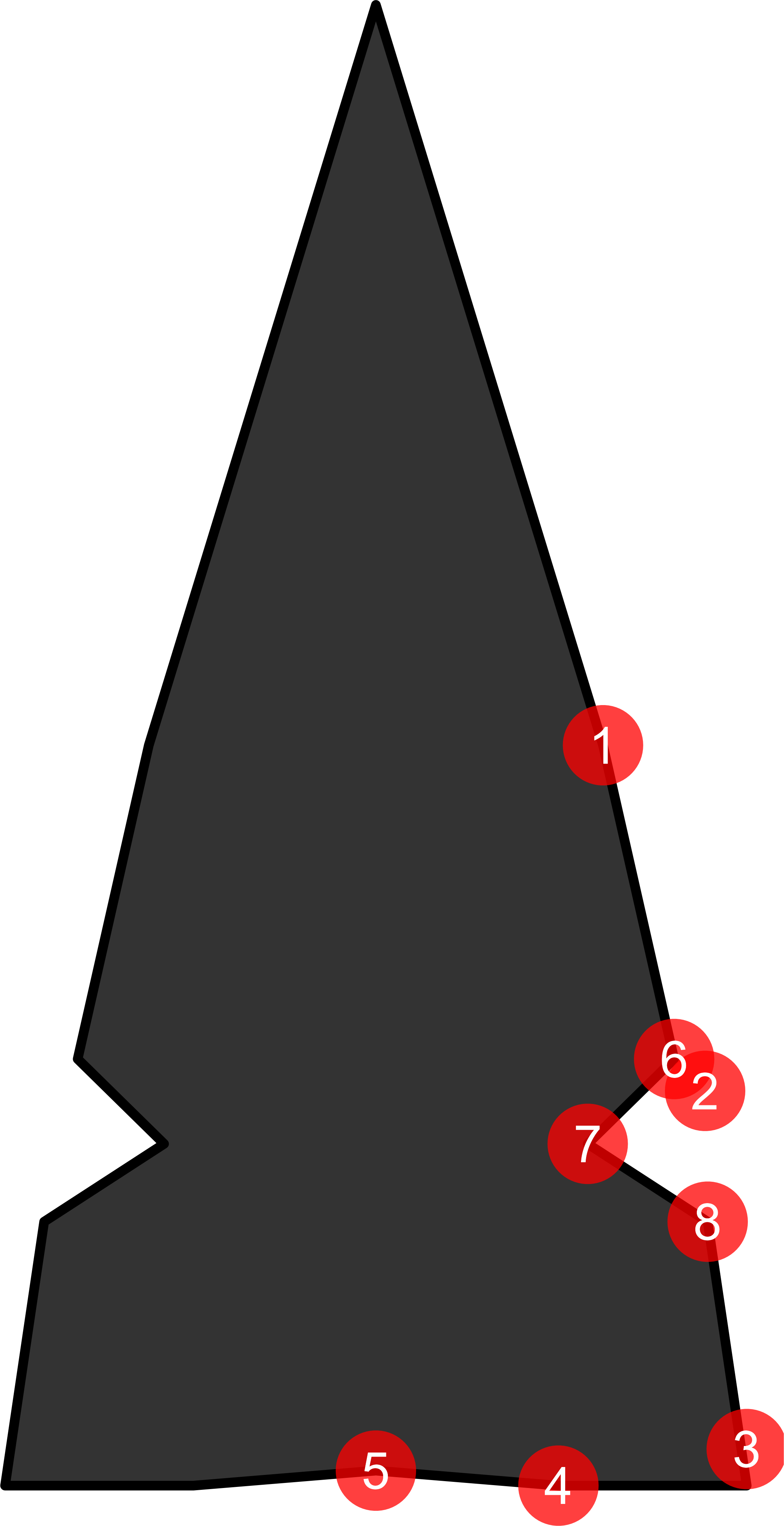
This procedure uses one corner of the projectile point as the target of the landmark analysis. As mentioned, this allows the analysis to incorporate damaged projectile points that are missing much of the rest of the projectile point. Landmarks were placed at key points (see Figure 3.2): halfway between the tip and basal corner, the basal corner, and the midpoint of the base. Two additional landmarks were placed in between each of these three landmarks. In addition to the five landmarks placed on all projectile points, side-notched projectile points had three landmarks placed at the top of the side-notch, the deepest part of the notch, and the bottom of the side-notch (see results section for more information). The curves function in TpsDig was used to accurately assign landmarks where the position was not obvious (.e.g., the corner of the base).
There were, however, many judgement calls to be made. In some cases it was difficult to judge where the bottom of the point transitioned to the side of the point when the point was curved. Notches could also have gradual transitions into the blade or base. For these reasons the initial batch of several hundred landmarks were reviewed for consistency and landmarks were adjusted as required. The TPS files were imported into R using the Momocs (Bonhomme et al. 2014) package. The Momocs package was used to apply GPA, and the aligned, scaled, and rotated landmarks were exported for additional analysis.
3.3.2 EFA
EFA analysis requires whole shape outlines. These can be created automatically in the Momocs package from imported image masks (black backgrounds with white objects). One potential pitfall for projectile points outlines is that some projectile points have asymmetric shapes as mentioned earlier when describing aligning points. This can affect the analysis if not accounted for, as significant morphometric variation will be ascribed to the orientation of the projectile point.
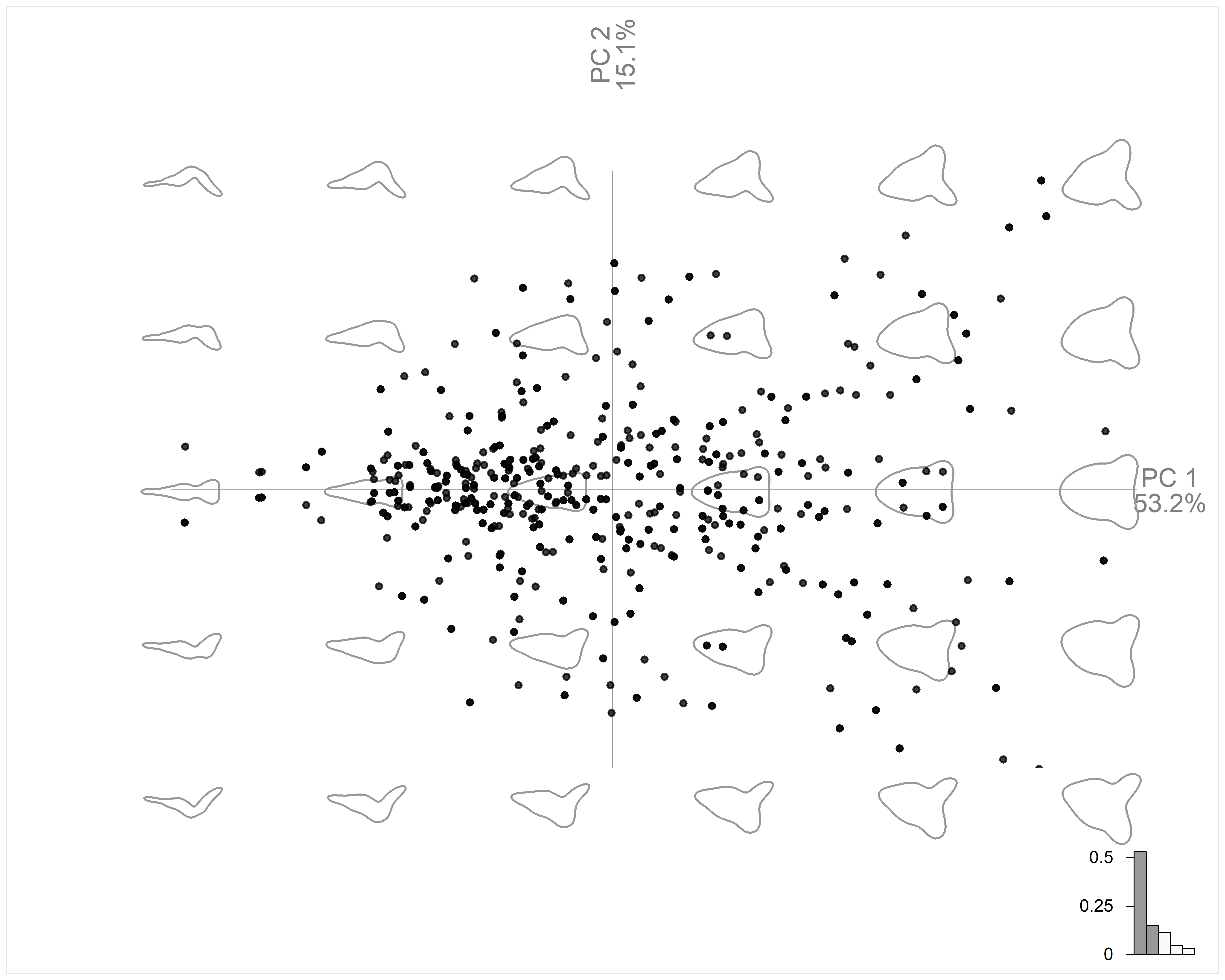
Of particular concern is the angle of the base. Many of the bases are not perpendicular to the vertical orientation of the projectile point. This variation can be manually addressed image by image. Another way is to use a GMM analysis. By examining the principal component (PC) space it is possible to determine which PC is related to shifts in the orientation of the base. Images that are aligned to one side of the PC can be identified en masse and flipped via command line instructions rather than manual adjustment to thousands of images. The Momocs package by default plots the morphometric variation along each PC axis as shown in Figure 3.3, which demonstrates that, in this example, PC2 is the orientation of the base. Once this process was completed, this axis of variation was eliminated which emphasizes important morphological attributes not related to the rotation of the point. Failing to take this or other issues related to the orientation of the projectile point can introduce considerable error into the analysis.
3.3.3 Dimensionality Reduction
PCA is commonly used for reducing the dimensionality of multivariate data. For a GMM example of PCA, an EFA analysis with only 10 harmonics will generate 40 columns of data without any clear indication whether any particular column is associated with more variation in the morphology. A PCA analysis can capture more than 95% of this variation with only 9 PCs using the data in this analysis. Not only is this a significant reduction in data, but the first two PCs capture 70% of the variation. This allows a simple biplot to show much of the variation in the multivariate data. PCA has been a mainstay in statistical analysis for decades, however, newer methods for reducing dimensionality have shown significant improvements.
A recently developed method called Uniform Manifold Approximation and Projection (UMAP) (McInnes et al. 2020) has proven to have many useful features that make it a better option than PCA in many cases where high dimensional data are being considered. UMAP is a dimensionality reduction technique that operates by creating a weighted graph (network) among a set of points based on high-dimensional data (in this case, EFA harmonics or GPA landmarks) with the strength of the ties between points defined based on their similarity across all dimensions. UMAP then projects this graph to a lower dimensional space that attempts to maximize the retention of the original graph topology in that lower dimensional space. UMAP as a method is designed specifically to attempt to capture a balance of local and global structure in complex high-dimensional data and thus, is a good fit for the kinds of information provided by GMM. The R umap implementation (Konopka 2020) produces just two dimensions from the input data. UMAP projections are primarily relied on in this analysis.
3.3.4 Spatial Analysis
A meaningful projectile point typology should have some correlation with geographic space (e.g., Azevedo et al. 2014; Hamilton et al. 2019). Two primary methods were used in this analysis to compare projectile point types across space: kernel density estimation (KDE) and a network community detection algorithm. KDE was used to create a smoothed estimate of the distribution of data. Hexagon grids were used to minimize edge effects. Each grid was 36 kilometers across, which roughly corresponds to one day’s travel on foot (Drennan 1984). While KDE is weighted towards locations with a higher number of points (in this case sites), this was undesirable for this analysis due to the uneven nature of data collection both for this study and for archaeology in general. Thus “hexagon binning” (Bischoff 2018, p. 59) was used where the data in each hexagon was aggregated and generated as a single point. This removed the effects of numerous sites in one location, such as Tonto Basin or Zuni.
The second method first involves a non-geographic method, network community detection, which was then projected across geographic space. First an archaeological similarity network was created by generating a weighted network graph using methods common in archaeological network analysis (M. A. Peeples and Roberts 2013). This was done by calculating the manhattan distance (more commonly known in archaeology as the Brainerd-Robinson distance) for each pair of sites standardized to a similarity score between one (identical) and zero (no similarity). A commonly used community detection algorithm is the Louvain method (Blondel et al. 2008), which works by merging groups together to find stable groups that maximize connections within a group while minimizing connections between different groups. This method was used to identify communities based on the projectile point typologies. These communities, which represent archaeological sites that have similar assemblages, were then plotted on a map.
3.3.5 Machine Learning
Given the size of the dataset used in this study, automating as much of the analysis as possible was essential. While geometric morphometric (GMM) methods were applied to quantify the shape variation of projectile points, machine learning models trained on these analyzed specimens were used to classify additional examples. Machine learning is particularly well-suited for this kind of task, as it enables efficient, consistent analysis at scale. However, it typically requires a labeled dataset for training—something this study provides through the prior GMM analysis.
Machine learning is increasingly common in archaeology (Bickler 2021), and its application to lithic analysis is gaining traction (e.g., Castillo Flores et al. 2019; Elliot et al. 2021; Lowe 2024; Nash and Prewitt 2016). At its core, machine learning involves training algorithms to identify patterns in data and make predictions (Bickler 2021, p. 186), though the implementation is often more complex in practice. This complexity brings potential pitfalls—particularly overfitting, where a model becomes too narrowly tailored to its training data and fails to generalize to new cases. To mitigate this, care was taken to follow the best practices recommended by Calder and colleagues (2022), including the use of unseen test data (15% of the total dataset) to validate model performance. For this study, the ResNet-18 model (He et al. 2016) was selected due to its strong accuracy, efficient training, and low computational demands. As a convolutional neural network, it extracts visual features across multiple layers and uses residual connections to support stable, efficient training. Its smaller size and speed made it particularly well-suited to the scale and goals of this analysis.
A pretrained model was used for all classification. The model had already been trained to extract image features and was fine-tuned on the projectile point dataset (described in a future section). Training was limited to 12 epochs to reduce the risk of overfitting, which occurs when a model learns patterns specific to the training data and fails to generalize to new examples.
3.4 Existing Typologies
The simplest approach to this analysis is to identify an existing typology that can be reliably replicated using a GMM approach. If GMM methods can successfully reproduce established typologies, they can enhance traditional classification by increasing consistency, reducing subjectivity, and enabling scalable, quantitative analysis of projectile points across large datasets. Moreover, replicating existing typologies with GMM at this scale would generate a labeled dataset large enough to train machine learning models capable of automating the classification process.
To implement this, it was first necessary to select a typology that could serve as a reliable reference for both the GMM training phase and subsequent machine learning classification. Excluding projectile point types idiosyncratic to specific projects—such as the Salado and Tonto types from the Roosevelt Platform Mound Study (Rice 1994)—there are nearly 70 projectile point types spanning the period of this analysis across four major typologies (Hoffman 1997; Justice 2002a; Loendorf and Rice 2004; Sliva 2006). While each of these typologies defines types based on some combination of morphological and temporal criteria, there is considerable overlap and inconsistency among them, making direct cross-typology comparisons difficult. Two main criteria guided typology selection: (1) broad geographic and temporal coverage across the study region, and (2) sufficient visual or physical representation of point types to support landmark-based analysis. Justice’s typology of projectile points in the Southwest (Justice 2002a) best met these requirements. It includes extensive illustrations and descriptions that span the entire Southwest and is further supported by a reference collection at the Museum of Northern Arizona that aligns well with Justice’s classifications.
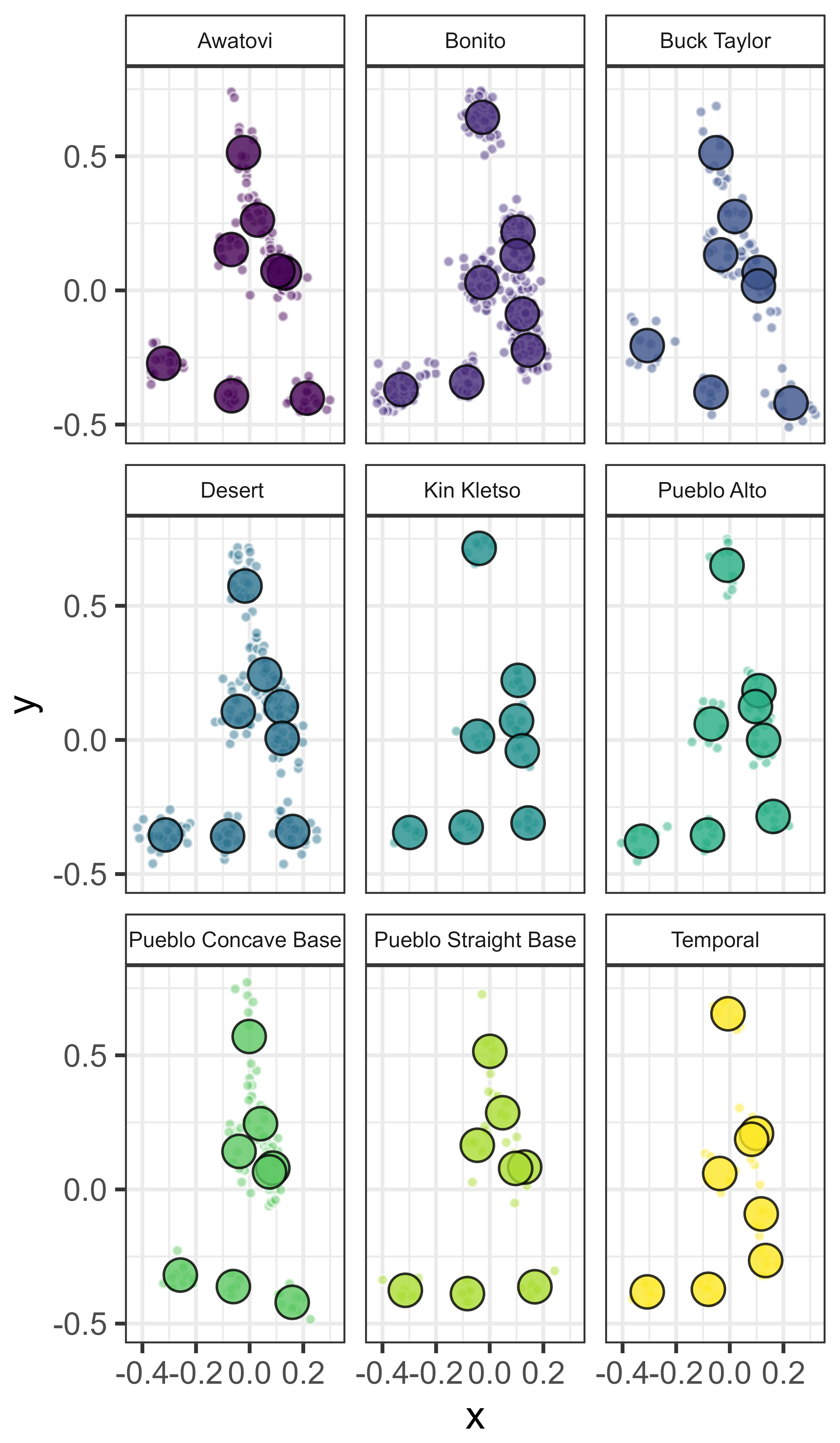
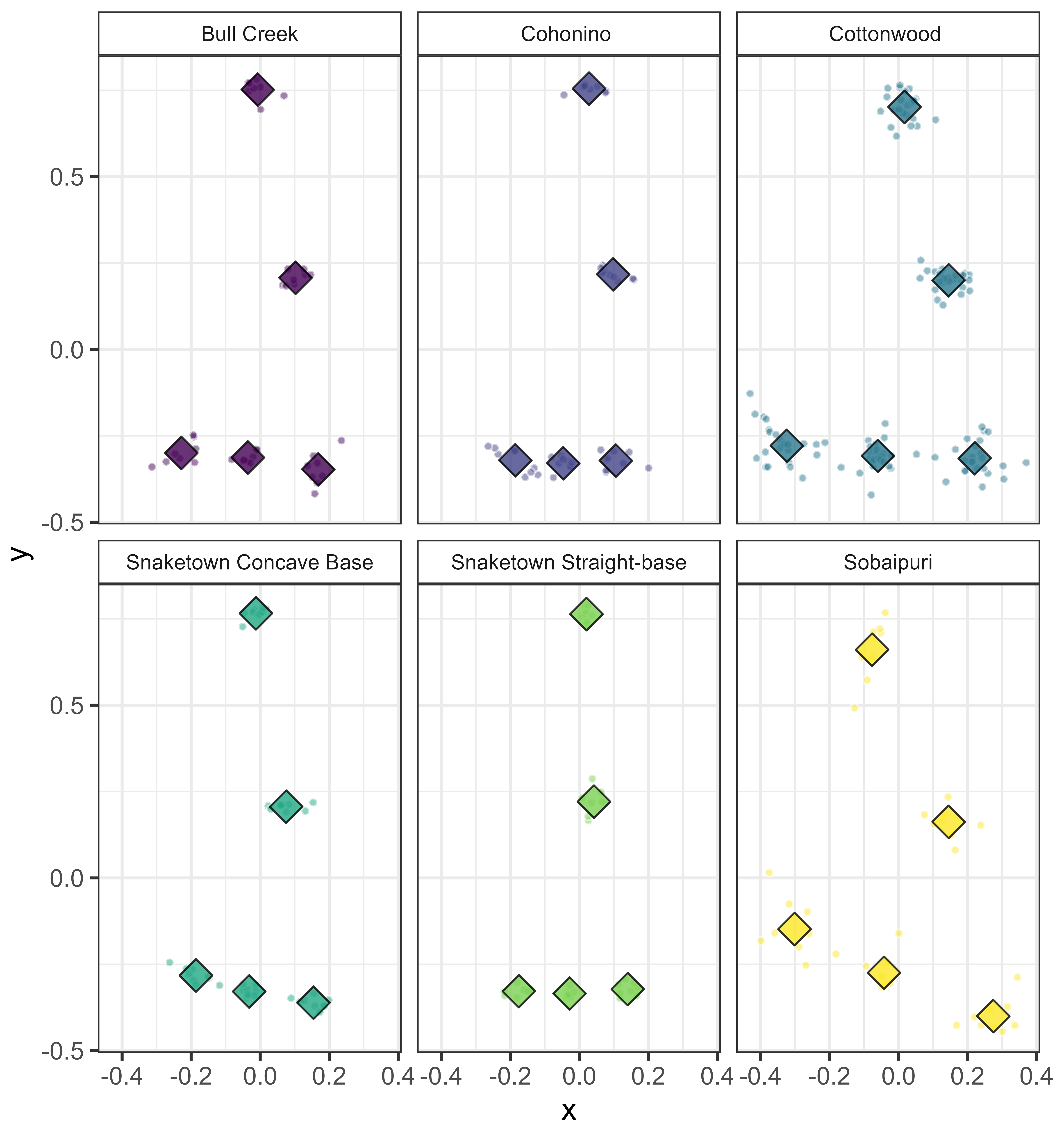
Because the number of landmarks differed between triangular and side-notched points, these forms were analyzed separately. Figures Figure 3.4 and Figure 3.5 show individual and mean landmark placements for several projectile point types. While there is some variation in notch shape for side-notched points, base shape is clearly distinguishable in both figures, with concave, convex, and straight bases visually separated.
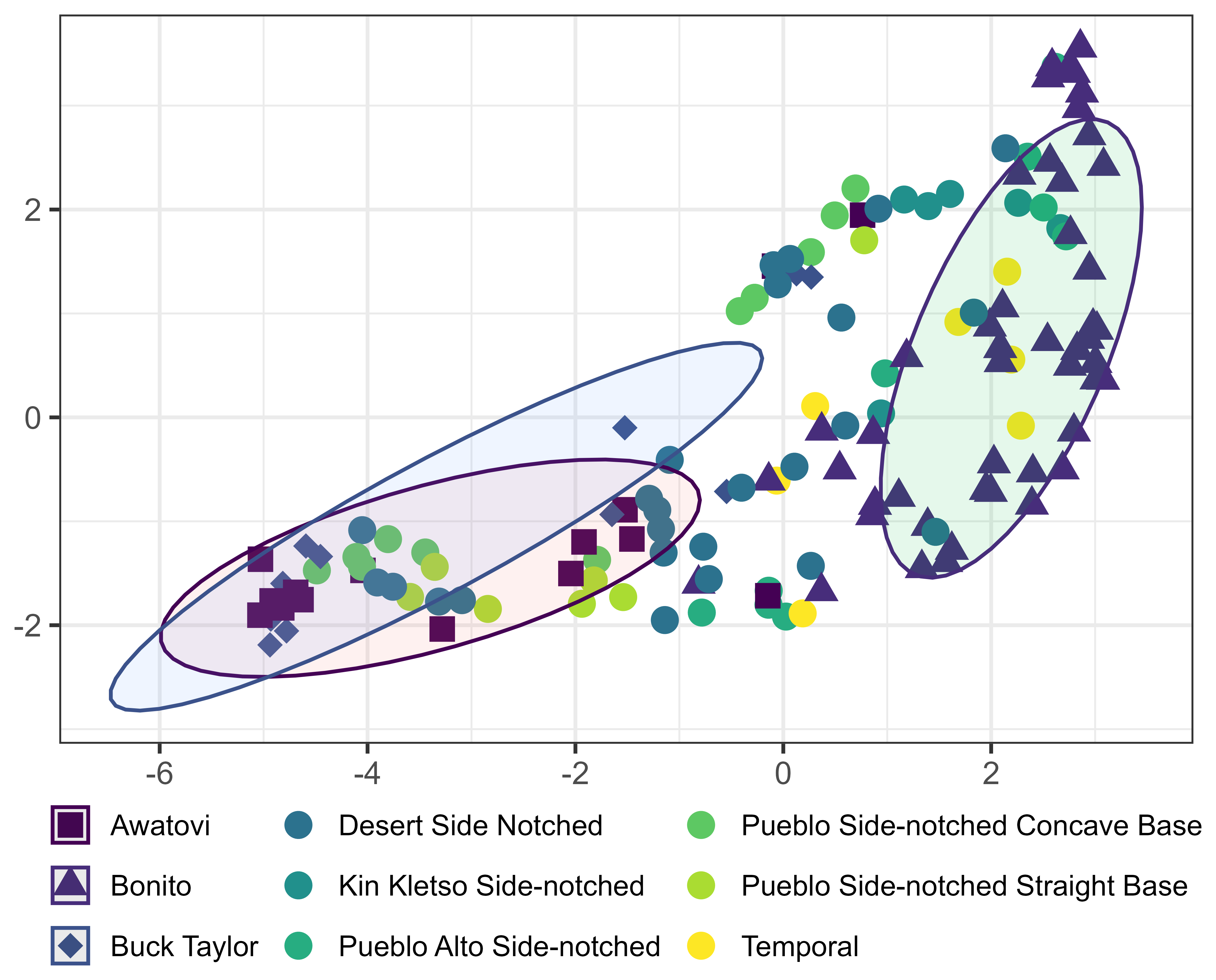
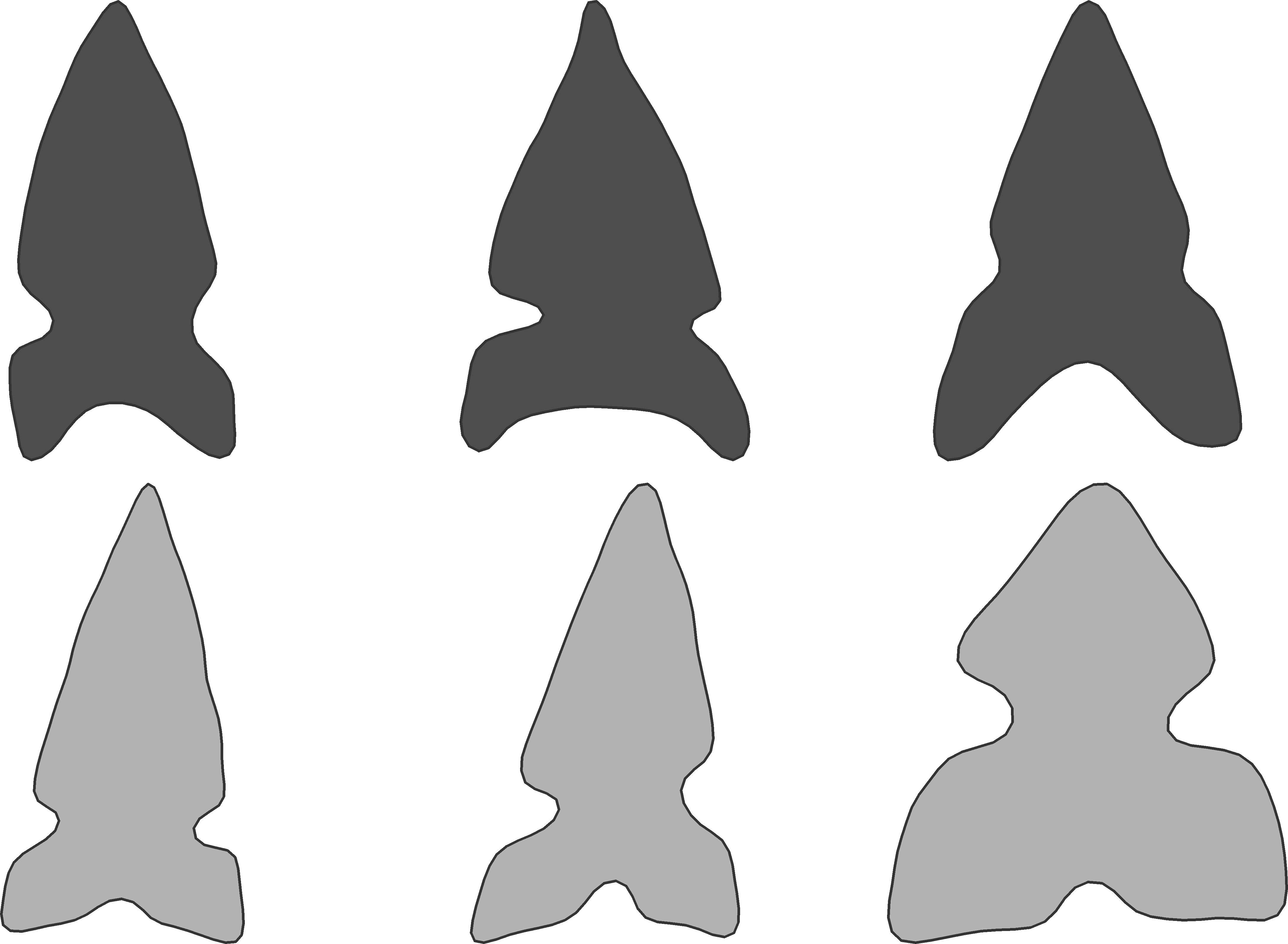
A UMAP projection of Procrustes-aligned landmarks for side-notched points (Figure 3.6) shows considerable overlap among point types, even when the ellipses are limited to 68% of the data (approximately one standard deviation). There are numerous outliers, but some types—including Awatovi, Bonito, and Buck Taylor—form relatively tight clusters with fewer outliers. These are also more easily distinguished visually. Awatovi points have basal notches, while Buck Taylor points are defined by deeply concave bases (see Figure 3.7). The GMM analysis appears to struggle to distinguish between basal notches and deeply concave bases, which likely contributes to this confusion, however, these attributes are important to some projectile point type definitions. Bonito points, which have convex bases that are uncommon in the dataset, also form a relatively distinct cluster.
The triangular point types show greater separation in the UMAP projection (Figure 3.8), although there are still several outliers. Sobaipuri points form one of the tightest clusters, but they still overlap with a number of other types.
The statistical validity of each group can be assessed using Hotelling’s \(T^2\) test (Hotelling 1931), which compares the means of groups across multiple related variables. This test is useful for evaluating whether the assigned groups are statistically distinct based on their multivariate representations—in this case, the UMAP coordinates. Table 3.3 shows comparisons between selected pairs of projectile point types, listing the number of points in each group (Type 1 Total and Type 2 Total), the Hotelling’s T-squared statistic, and the associated p-value. Only comparisons with p-values greater than 0.1 are shown to highlight cases where separation is not statistically supported. The p-value represents the probability of observing a difference as large as the one measured (or larger), assuming there is actually no difference between the two groups.
The results show that most side-notched types are statistically distinguishable from one another based on the UMAP projection of Procrustes-aligned landmarks. However, Table Table 3.3 highlights the exceptions—pairwise comparisons among side-notched types where Hotelling’s \(T^2\) test produced p-values greater than 0.1, indicating insufficient evidence for clear separation. While some comparisons, such as Bonito and Kin Kletso Side-notched, approach significance, each of the listed types has at least one other group with which it overlaps morphometrically. In contrast, triangular types show stronger overall separation, though the comparison between Bull Creek and Snaketown Triangular Concave Base did not yield a statistically significant result. These findings are somewhat unexpected given the simpler outlines of triangular points, but they suggest that side-notched features may introduce variation that is not consistently captured in the GMM-based analysis.
| Type 1 (n) | Type 2 (n) | T² | P-value |
|---|---|---|---|
| Awatovi (15) | Buck Taylor (11) | 0.33 | 0.85 |
| Awatovi (15) | Pueblo Side-notched Concave Base (11) | 1.86 | 0.42 |
| Bonito (48) | Temporal (7) | 4.49 | 0.12 |
| Buck Taylor (11) | Pueblo Side-notched Concave Base (11) | 3.78 | 0.19 |
| Desert Side Notched (25) | Pueblo Side-notched Straight Base (7) | 2.02 | 0.39 |
| Kin Kletso Side-notched (6) | Temporal (7) | 5.62 | 0.13 |
| Pueblo Alto Side-notched (9) | Temporal (7) | 0.39 | 0.84 |
| Bull Creek (8) | Snaketown Triangular Concave Base (9) | 2.85 | 0.30 |
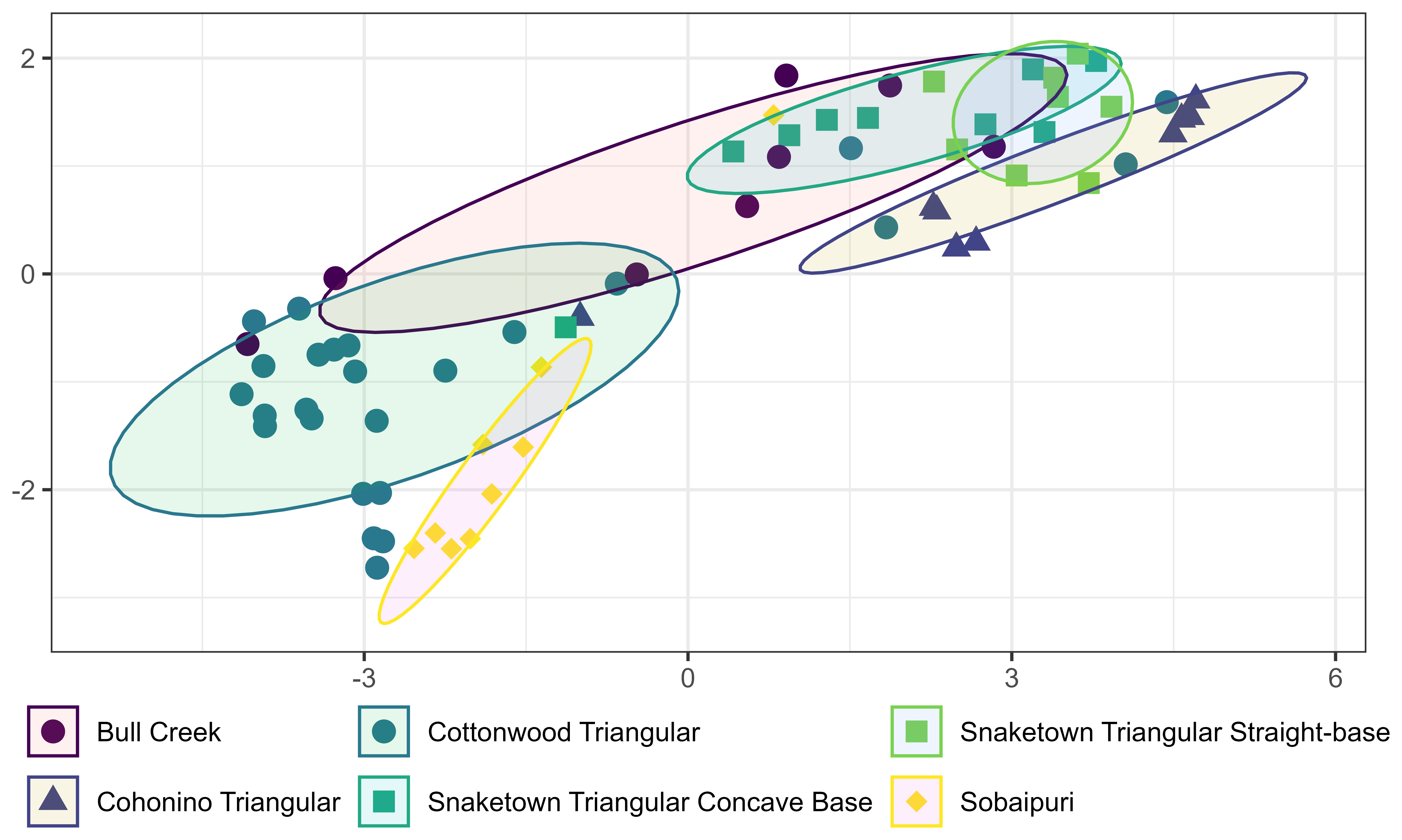
Figure 3.9 highlights a key issue with using typologies for projectile points. The figure shows continuous morphological variation across the dataset, with no clear boundaries between types. While many projectile points appear visually distinct, there is often a morphological continuum that isn’t immediately obvious. For example, the difference between a basal notch and a concave base may be gradual when enough examples are considered. Similarly, the distinction between concave and straight bases can range from obvious to nearly indistinguishable. Typological categories can be useful for organizing and interpreting data, but it’s important to recognize that they often oversimplify and obscure meaningful variation within and between groups.
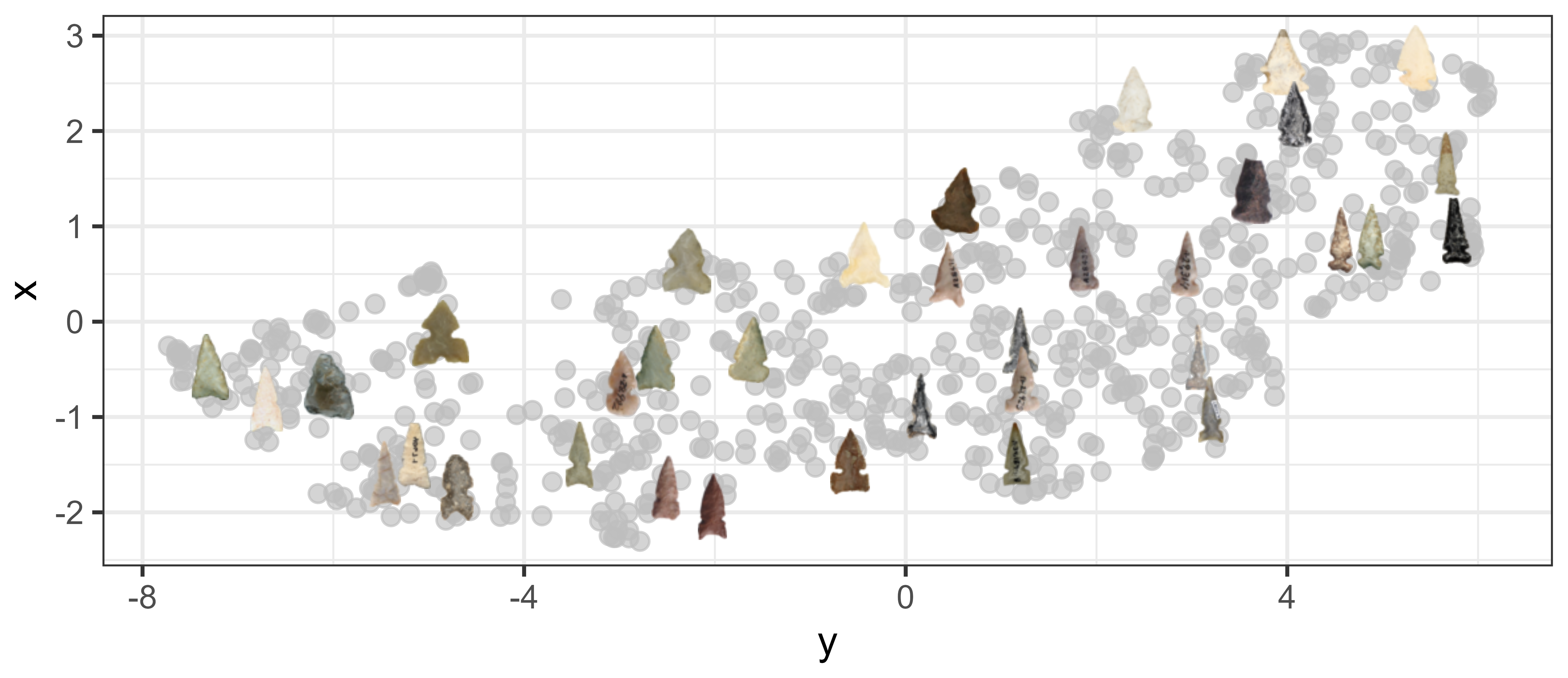
Overall, this analysis suggests that traditional regional typologies do not adequately capture patterns of morphological similarity in projectile point design—at least not for side-notched points. The overlain projectile point images in Figure 3.9 show that points located near each other in the projection are morphologically similar, but reducing the variation to a manageable number of clusters requires an impractically high number of groups. Ideally, landmark data alone would allow points to be assigned to clear, well-separated types, but that is not the case here. A hybrid approach could be taken, where easily distinguishable types are retained and new types are created as needed. However, to maintain consistency throughout the analysis, existing typological categories were set aside in favor of a strictly attribute-based classification.
3.5 Attribute-based Typology
Based on the existing typologies for late prehistoric projectile points in the region (Loendorf and Rice 2004; Rice 1994; Tagg 1994; Thomas 1981), several attributes were chosen for this analysis. These typologies, while not always consistent, reflect long-standing expert observations about morphological variation and regional traditions. Selecting attributes from them allows for continuity with prior research and provides a basis for testing whether quantitative methods like GMM can replicate or refine traditional classifications. These attributes are:
Point form (e.g., triangular vs. side-notched)
Base shape (e.g., concave vs. convex)
Basal notch (e.g., presence/absence)
Notch height (for side-notched points)
Serration (presence/absence)
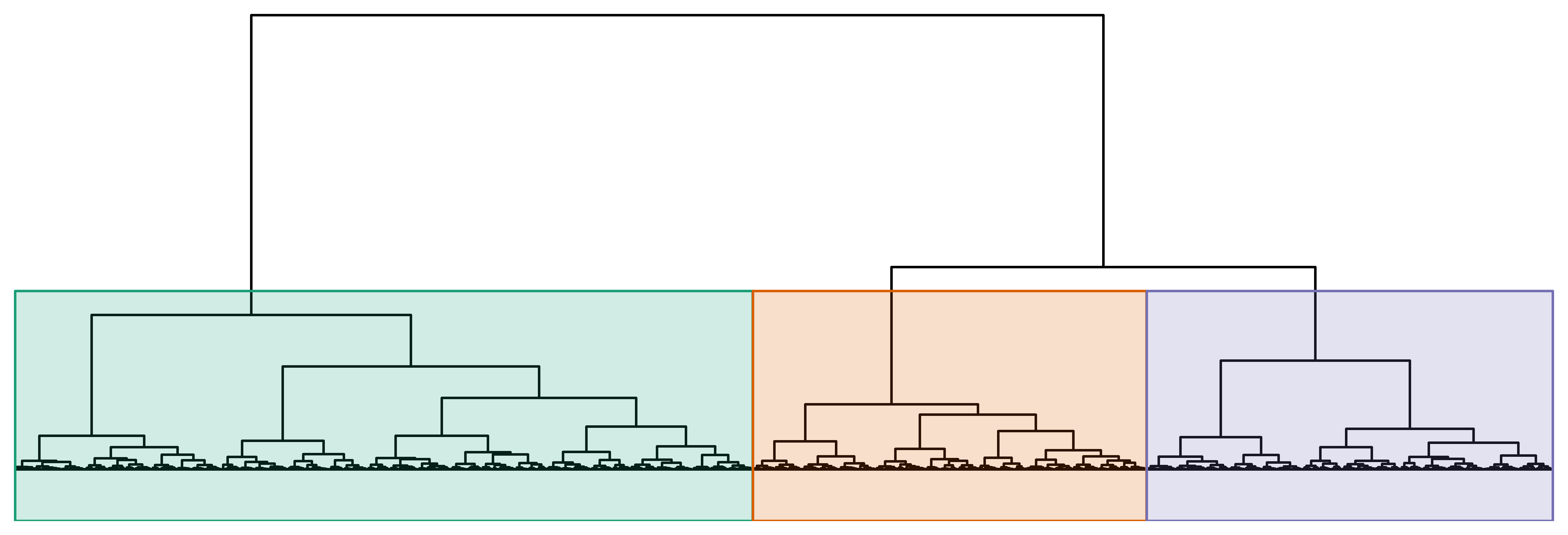
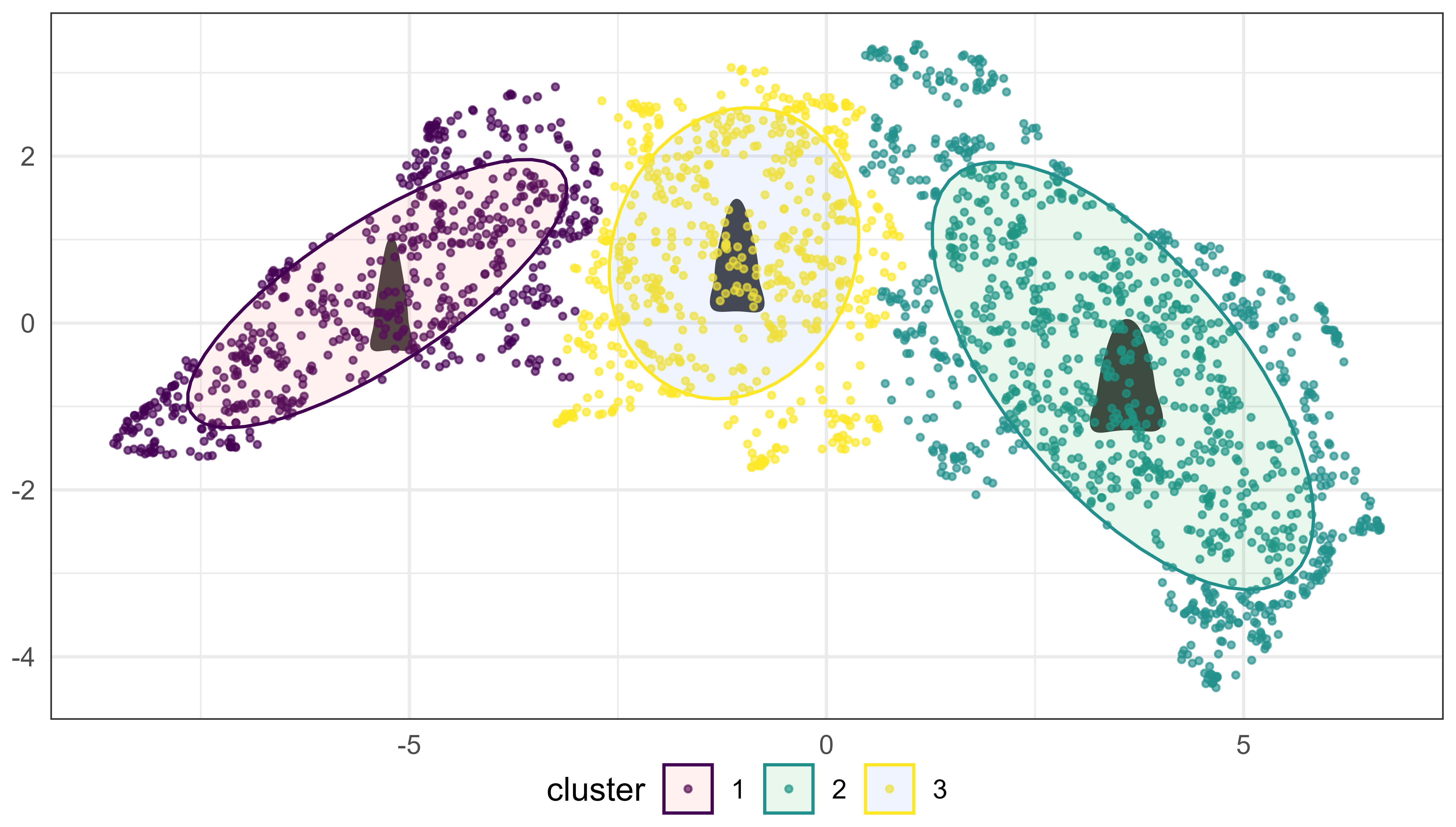
One additional attribute was also considered: three morphologically determined shape clusters. All projectile points were grouped into three clusters based on overall shape using elliptical Fourier analysis (EFA), which was chosen because it captures the entire outline of each point. Landmark analysis was initially preferred, as about one-fourth of the points had damage that distorted their outlines. While in many cases this damage did not significantly affect the EFA results, all assignments were reviewed for consistency, and reassignments were made when necessary. Hierarchical cluster analysis was applied to the UMAP results derived from the EFA coefficients (Figure 3.13), and the number of clusters was selected by identifying major branches in the resulting dendrogram.
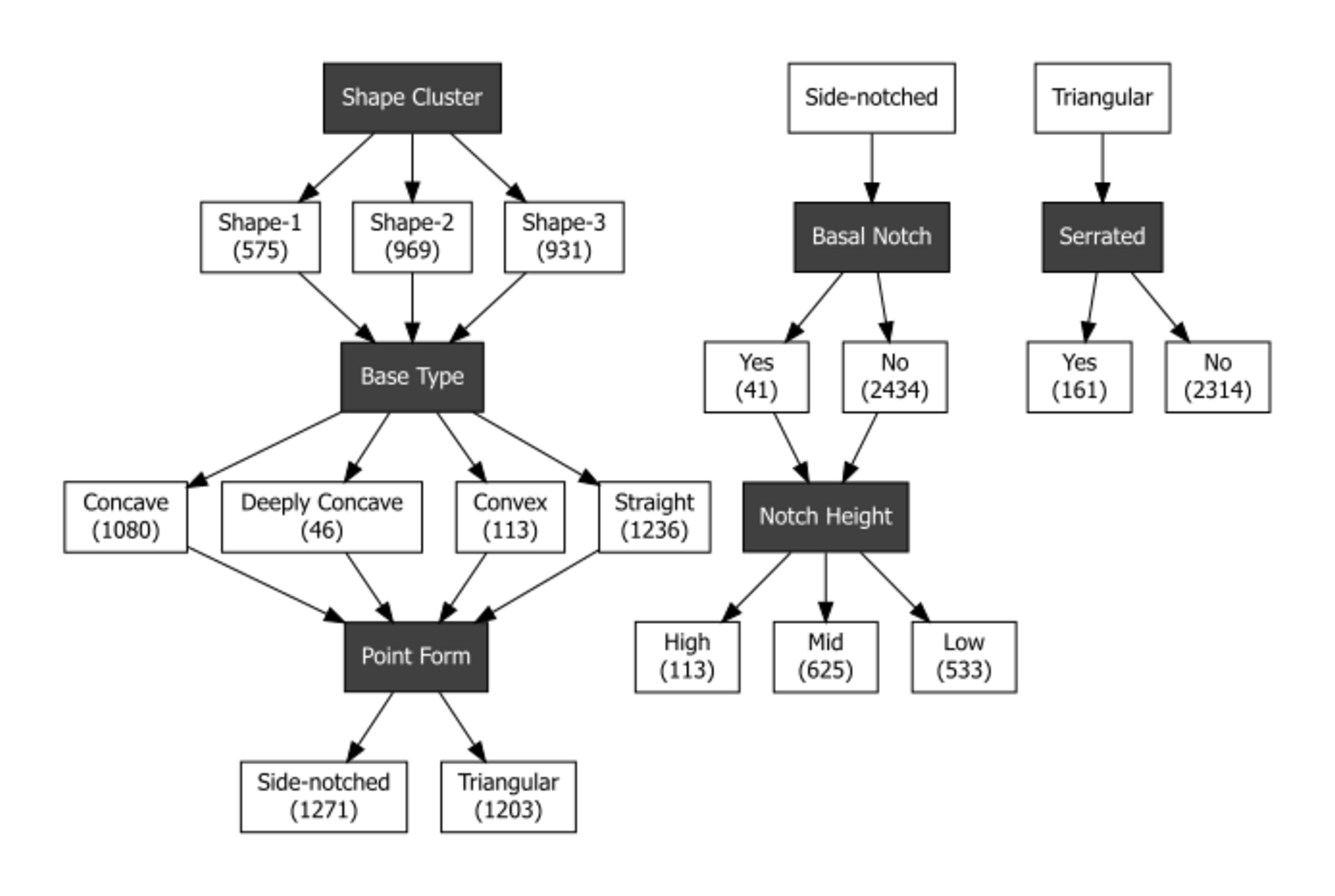
With the five attributes mentioned above plus the addition of the shape clusters, the projectile points were assigned to attribute-based types as shown in Figure 3.10. Notably, less than 2% of side-notched points were serrated, while almost 11% of triangular points were serrated. Given this and to reduce the number of potential types, serration was only considered for triangular points. This also matches the projectile point typologies as none of the side-notched types considered in this analysis are defined by their serration.
The identification of each projectile point attribute is described below. Where appropriate, GMM methods were used for attribute assignment, with additional verification through machine learning. Machine learning models were trained for all attributes except for distinguishing triangular versus side-notched points, which were initially identified during data collection.
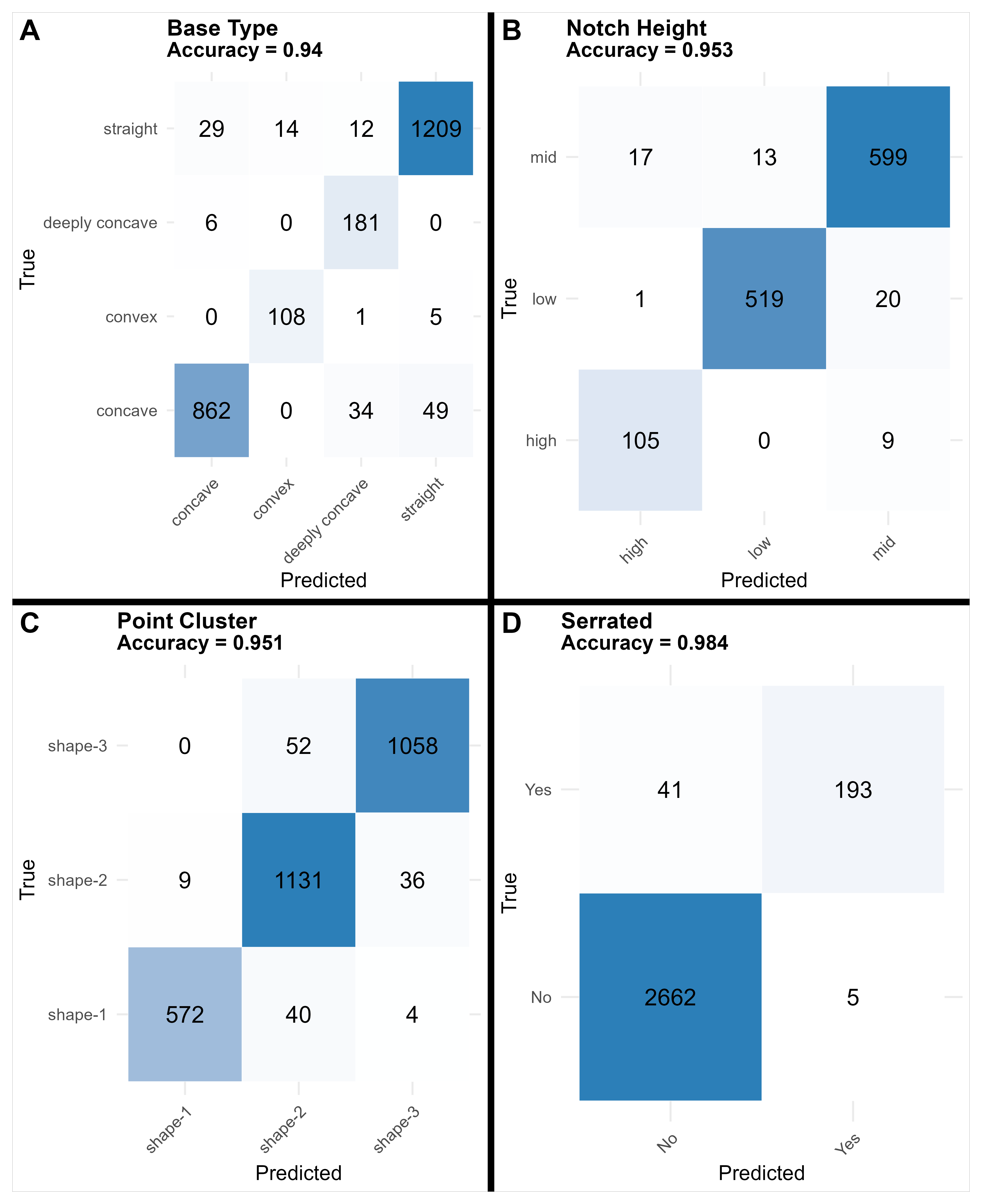
Each model was developed with three main purposes: (1) to assign attributes to projectile points where values were missing, (2) to evaluate and correct inconsistencies in initial assignments, and (3) to provide trained models for use in future analyses. Model performance was assessed by comparing predicted attributes to initial labels across the full dataset. As shown in Figure 3.11, the classification accuracy ranged from 93.7% (base type) to 98.4% (serration). These results reflect internal consistency rather than out-of-sample performance.
To evaluate initial assignments, each trained model was used to predict attribute values for all projectile points. Any mismatches between the predicted and original assignments were flagged for manual review. This process revealed numerous inconsistencies in the original data, particularly for base type and point cluster, which were corrected where appropriate. After corrections were made, models were retrained, significantly improving overall assignment quality and model reliability.
Further details on machine learning implementation, including architecture and training parameters, can be found in the supplementary Python code and Appendix B.
The determination of side-notched points vs. triangular points was done visually as the landmark data required predetermining whether the point had notches. Likewise, the basal notches and the serration were visually assigned as well, as the GMM methods struggled to differentiate deeply concave points vs. basal notched points as well as serration. A machine learning model was trained on serration primarily to check assignments for errors.
The point clusters were determined by creating outlines of all projectile points and conducting an EFA analysis. This generates fourier coefficients which were subjected to a UMAP transformation (Figure 3.13) and a subsequent hierarchical clustering analysis. Three major branches formed in the tree plot (Figure 3.12), and thus three clusters were chosen for assignments. Hotelling’s \(T^2\) tests indicate all three clusters can be clearly differentiated. A machine learning model was created for the shape clusters and used for validation. The three clusters are primarily differentiated by height and width ratios.
The landmark data were best suited for assigning the base type into the categories used for this analysis. Angles between the third and fifth landmarks were calculated and initial visual assignments were used to gauge appropriate angles for assigning categories. These four categories were used for the analysis with the following assignments for angles (0 degrees represents horizontal):
- deeply concave < -12
- concave < -5 & >= -12
- straight >= -5 & <= 5
- convex > 5
Assignments were then visually checked for errors and modified as needed. A machine learning model was trained as described above and used to assign points that were not landmarked. Again, points were visually checked and modified as needed.
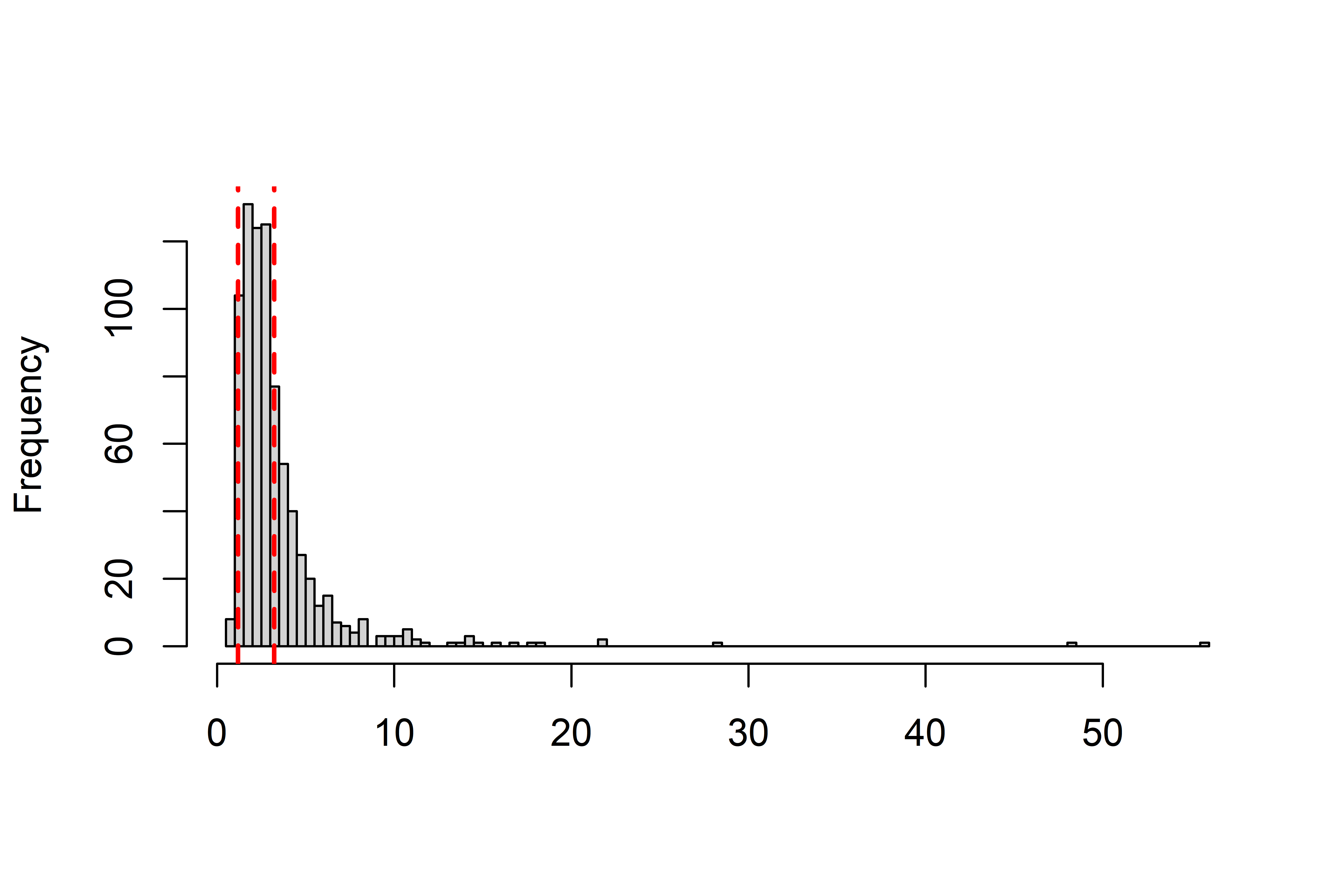
Notch heights were determined using landmark data to assess the relative vertical position of the notch. Specifically, the ratio of the distance from the first landmark to the bottom of the notch to the distance from the third landmark to the base was calculated for each point. This ratio served as a standardized measure of notch height, independent of overall point size. A histogram of these ratios (see Figure 3.14) revealed a clear central distribution, with most notches falling within a well-defined middle range. To classify the points into low, mid, and high notch categories, quantile-based cutoffs were applied. High-notch points were defined as those above the 0.67 quantile—approximately one standard deviation above the mean—capturing the upper end of the distribution. Low-notch points were defined as those below the 0.025 quantile, a threshold chosen based on a sharp drop observed in the histogram, indicating a natural break in the data. All remaining points were classified as mid-notch. This approach allowed for the classification of notch position in a way that reflects both the overall distribution and notable discontinuities in the data.
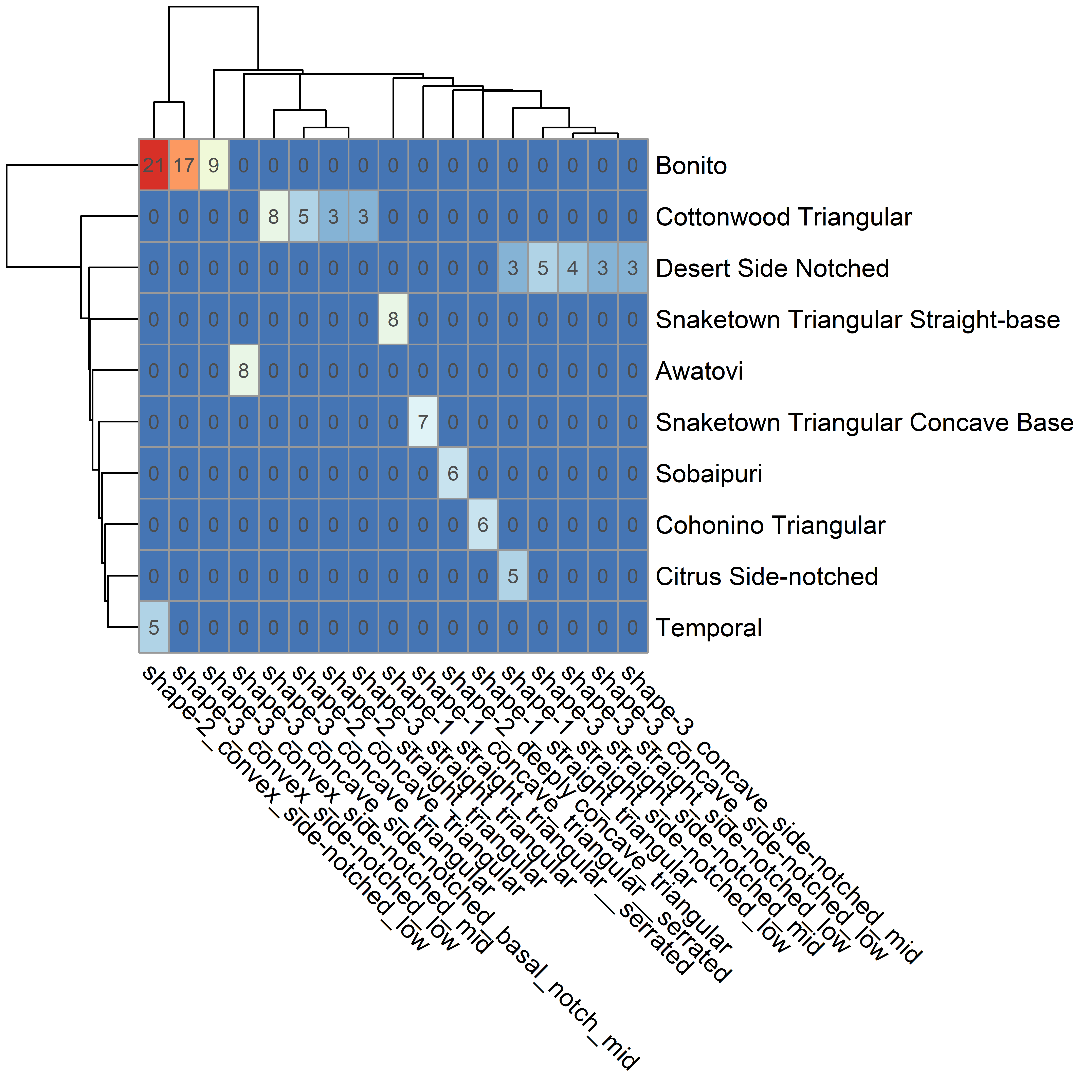
Once all attributes were assigned and visually checked for consistency, the projectile point type was assigned by following the decision tree. The number of attributes involved resulted in 45 side-notched types and 20 triangular types. Six of these types had only a single projectile point. Four of these were side-notched types with a basal notch. Two of these were triangular points with a convex base. Side-notched types had a maximum of 129 projectile points with a median of 11. Triangular types had a maximum of 249 with a median of 20. Figure 3.15 demonstrates how these attribute-based types align with the existing typologies previously tested with GMM. The attribute-based assignments are far better at determining the original assignments than GMM alone. One exception where one attribute-based type was assigned to multiple existing types is caused by a missing attribute for Temporal projectile points, which are defined as having extra notches. This attribute was not considered in this analysis. The other exception is Citrus side-notched, which overlaps somewhat with Desert side-notched. This is not surprising as the Desert side-notched type is somewhat vaguely defined.
Hotelling’s \(T^2\) tests indicate that most types were easily distinguishable. There were some exceptions, shown in Table 3.4. This table shows test results with p-values above 0.1. Groups with fewer than 10 projectile points were not included in these tests. In the cases where the groups were not easily distinguished via Hotelling’s \(T^2\) tests, the attributes were closely related. For example, types that were identical with the exception of serration were harder to distinguish. In other examples, most attributes were similar. Only 4 of the 12 paired groups had more than 1 attribute that was different than the comparison group, the rest only had 1 different attribute. Each individual attribute, however, when considered as a group, is easily distinguishable via Hotelling’s \(T^2\) tests.
| Group 1 (n) | Group 2 (n) | T² | P-value |
|---|---|---|---|
| shape-1_concave_side-notched_low (26) | shape-1_straight_side-notched_low (45) | 0.39 | 0.82 |
| shape-1_concave_side-notched_mid (29) | shape-1_deeply concave_side-notched_mid (11) | 1.04 | 0.61 |
| shape-1_concave_side-notched_mid (29) | shape-1_straight_side-notched_mid (13) | 0.14 | 0.93 |
| shape-1_deeply concave_side-notched_mid (11) | shape-1_straight_side-notched_mid (13) | 0.55 | 0.77 |
| shape-1_deeply concave_side-notched_mid (11) | shape-2_concave_side-notched_mid (46) | 3.21 | 0.22 |
| shape-2_concave_side-notched_high (10) | shape-3_concave_side-notched_high (12) | 0.79 | 0.69 |
| shape-2_concave_side-notched_mid (46) | shape-2_straight_side-notched_mid (56) | 3.39 | 0.19 |
| shape-3_concave_side-notched_mid (61) | shape-3_deeply concave_side-notched_mid (23) | 0.62 | 0.74 |
| shape-1_concave_triangular__serrated (17) | shape-1_deeply concave_triangular (27) | 1.70 | 0.44 |
| shape-1_straight_triangular (103) | shape-2_concave_triangular__serrated (13) | 3.26 | 0.20 |
| shape-2_concave_triangular (76) | shape-3_concave_triangular__serrated (10) | 0.89 | 0.65 |
| shape-3_concave_triangular (88) | shape-3_concave_triangular__serrated (10) | 2.73 | 0.26 |
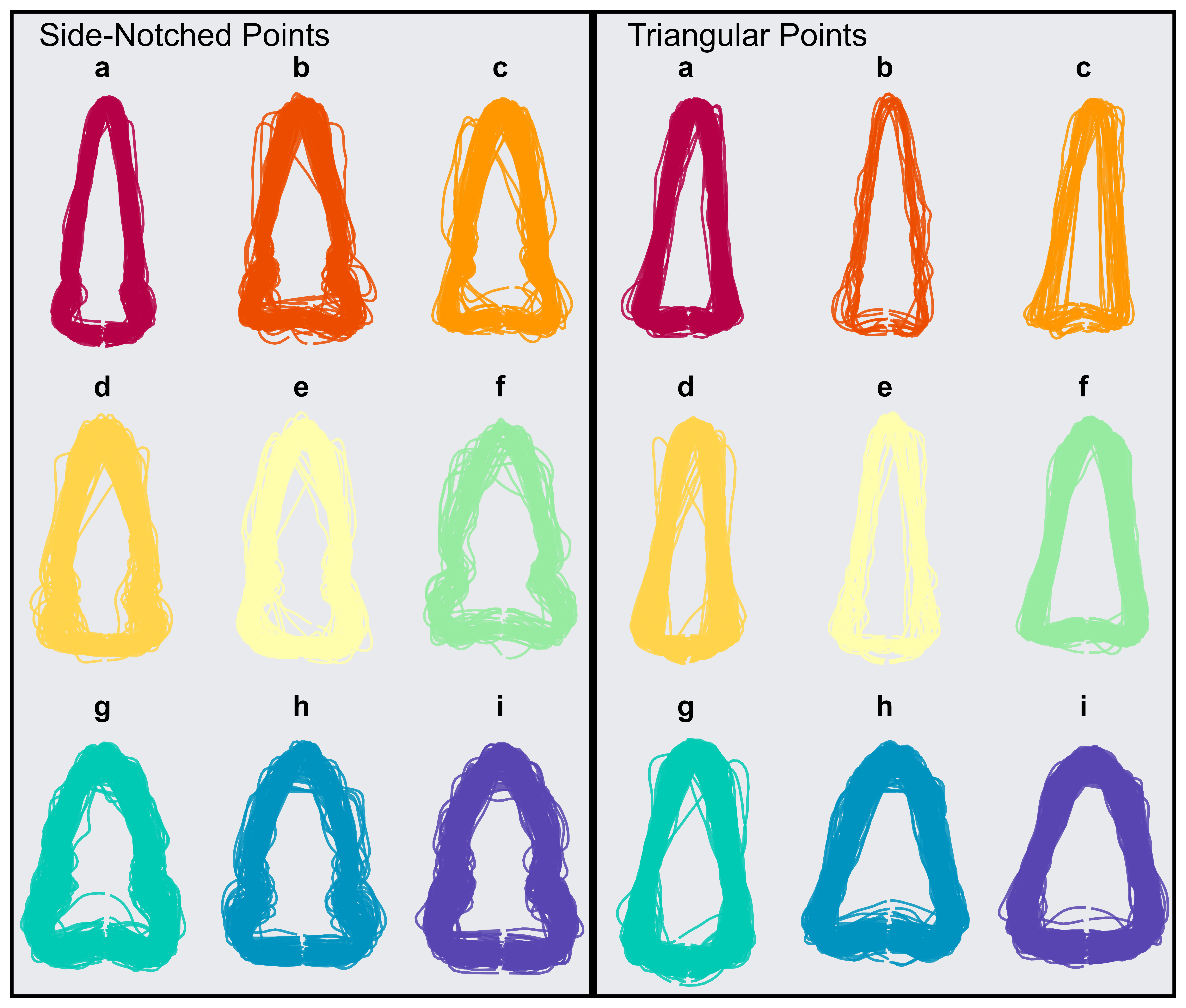
Figure 3.16 shows the projectile point outlines for some of the most common types used in this analysis. The shape outlines have been scaled and rotated using an automated GPA process in the Momocs package. These types represent over 75% of the total number of assigned projectile points in the database. Several of these points would be easy to visually discriminate, while others are noticeably different but would be difficult to discriminate from a cursory visual examination. The attribute approach used here using a combination of GMM methods and visually identified attributes supplemented with machine learning for replication and additional validation provides an alternative to traditional typological methods. What is yet to be determined, is whether these types can usefully be applied in a regional analysis.
3.6 Geographic Clustering
If, as argued earlier, cultural factors play a significant role in the variation of projectile point morphology, then it is unreasonable to expect a random distribution of projectile point types across such a large region. While some degree of randomness is expected—especially given the extensive population movements discussed previously—a complete lack of spatial patterning would undermine the assumption that point forms are culturally meaningful. In that case, the validity of using projectile point morphology to infer cultural or regional patterns would be questionable. Figure 3.17 shows the distribution of the side-notched projectile point types and Figure 3.18 shows the triangular types. These maps use the KDE hexagon bins previously described.
Essentially these figures show the general distribution of the projectile point types by showing the frequency of each projectile point type relative to the total number of points in each cell. The KDE function smooths the values to provide a clearer representation of density variations across the study area, reducing the impact of local anomalies and highlighting broader spatial trends. Pronounced geographic patterning is evident, with distinct clusters of specific projectile point types emerging across the study region. These spatial trends reflect underlying social, technological, and environmental factors that influenced the production, use, and exchange of projectile points. The strongest gravitational centers are in the Sinagua and Mogollon regions. Curiously, the Zuni regions have an even mix of projectile point types with no strong tendency towards any particular style.
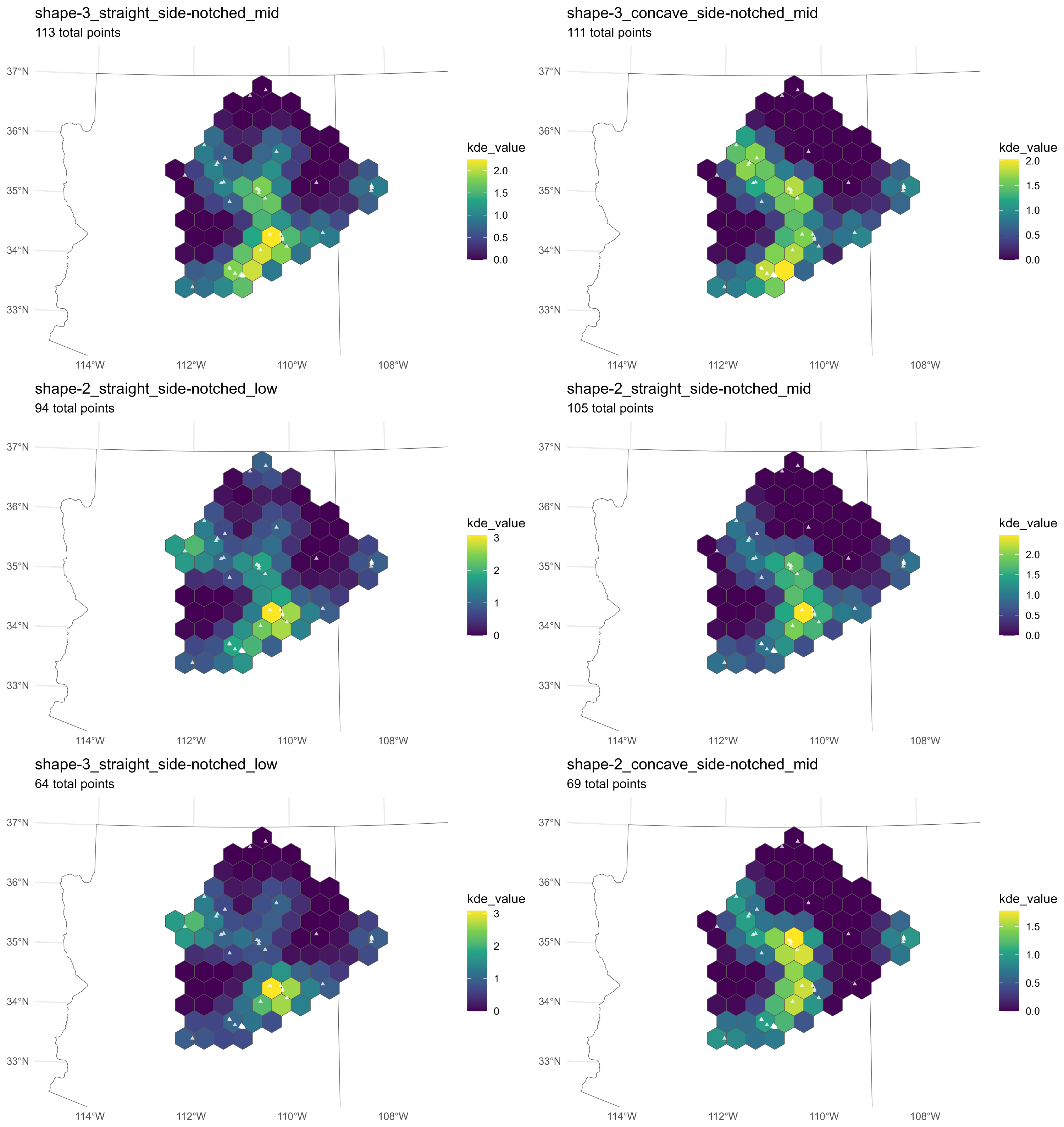
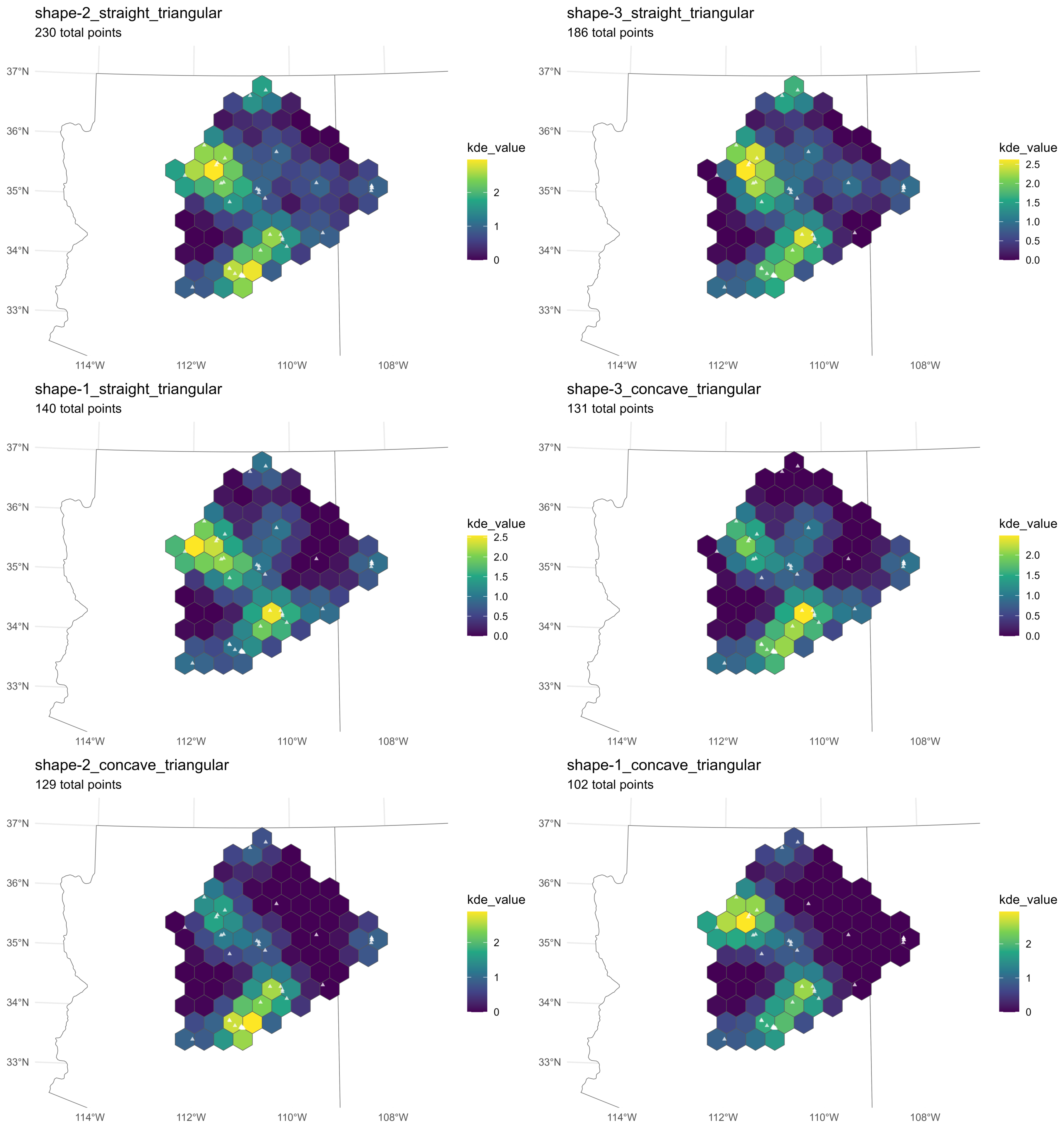
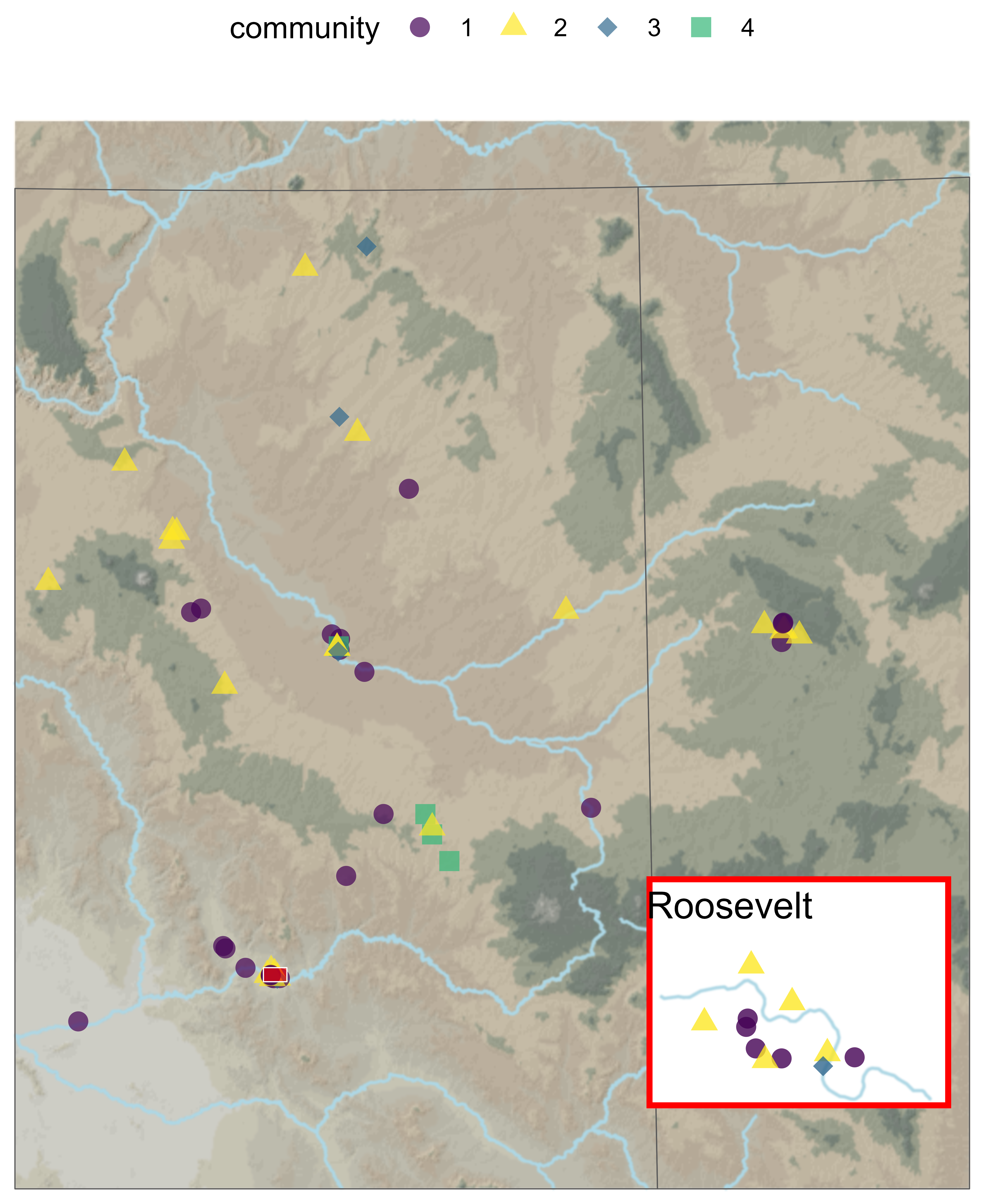
Figure 3.19 shows a map of the project area with sites assigned to communities based on the network clustering method described earlier. Sites are grouped into communities according to similarities in projectile point assemblages, using the newly defined attribute types. Weak connections—-those below the 0.75 similarity quantile-—were excluded, and isolated sites with no ties are not shown.
Communities 3 and 4 are small, with five and four sites respectively. Most of these sites are relatively close in proximity, with the exception of the Community 3 site in the Roosevelt region shown in the Figure 3.19 inset. Most sites fall into communities 1, or 2, which show a general east-to-west distribution, although with significant mixing. Hohokam sites appear to predominantly fall into Community 1, but many other sites share projectile point styles and fall in this community. Community 2 is concentrated in the northern portions of the region, but with a major presence in the Roosevelt region as well. Notably, the Roosevelt inset in Figure 3.19 highlights sites from different communities. While several sites belong to community 1, several other outlying communities belong to Community 2 and one belongs to Community 3. The diversity in the Roosevelt area points to complex interaction patterns that are explored further elsewhere [Bischoff (2023a); Chapter 4 of this dissertation]–see also the work by Watts (2013).
These two methods of examining the spatial distribution of the projectile point types demonstrate spatial patterning throughout the project area and successfully demonstrate that the adopted attribute-based projectile point types used in this analysis produce meaningful results in a regional study. Further analysis, particularly in combination with other types of material culture would improve our understanding of these patterns, however, these results are enough to demonstrate the utility of the methods described in this chapter.
3.7 Discussion
The analysis confirms that while GMM methods, especially elliptical Fourier analysis (EFA), are valuable for capturing overall shape, they struggle with specific morphological features like side notches and basal indentations (Bischoff 2023b; Bischoff and Allison 2020; Okumura and Araujo 2016). Landmark-based methods improve this (F. L. Bookstein 1997; Shott and Trail 2010), but are time-consuming and still fall short in distinguishing features like basal notches versus deeply concave bases—a limitation noted in prior morphometric studies (Charlin and González-José 2012; Petřík et al. 2018).
Importantly, this analysis found that continuous variation is the norm in projectile point morphology (Anderson et al. 2010; Archer et al. 2015; Barton 1988; Bretzke and Conard 2012; Lycett and Cramon-Taubadel 2015), which complicates efforts to fit points into rigid typological categories. Despite these challenges, GMM has been shown to be highly effective in identifying broad regional shape patterns (Buchanan and Collard 2010; Charlin and González-José 2012; Okumura and Araujo 2016; Petřík et al. 2018; Selden 2022), and this study contributes additional support for its use in regional analysis.
Furthermore, emerging approaches that integrate machine learning with GMM have shown promise in improving classification efficiency and accuracy (Bonhomme et al. 2023; MacLeod 2018). Several studies have successfully combined the two methods to automate the classification of lithic forms at scale (Courtenay et al. 2019; Maté-González et al. 2023). In this study, machine learning models also provided critical validation checks, catching inconsistencies in initial attribute assignments and supporting a scalable, replicable workflow.
The spatial patterns identified in this analysis reinforce previous findings that projectile point types correspond with cultural and linguistic boundaries (Ryan 2017; Sliva 2006; Whittaker and Bryce 2017) and migration-related artifact distributions (Bischoff 2023a; J. J. Clark 2001; Elson 1996; Spielmann et al. 1998; Wood 2000). As demonstrated in Chapter 4 of this dissertation, projectile point networks correspond with material culture clusters, especially in areas like the Roosevelt region, where immigrant communities have previously been documented.
3.8 Conclusion
This analysis of over 3,000 projectile points from 81 sites across various culture areas—Ancestral Pueblo, Hohokam, Mogollon, and Sinagua—demonstrates that regional-scale projectile point analyses can be efficiently conducted using geometric morphometric (GMM) and machine learning techniques. The findings show that an attribute-based approach to categorization is more effective than relying solely on overall shape, particularly when dealing with morphologically complex forms like side-notched points. The results also confirm that 2D image data alone can be sufficient for exploring regional variation in projectile point distributions, making this method highly accessible and cost-effective.
A key contribution of this study is the development and testing of a classification system based on discrete morphological attributes such as base shape, notch height, and serration. While these attributes were drawn from Southwest typologies, they are not regionally specific and have broad applicability to other regions where similar projectile point forms are found. Because the attributes are based on generalizable aspects of shape and form rather than on specific type names, they can be adapted to different contexts, enhancing the utility and flexibility of the method.
Moreover, the integration of GMM and machine learning not only improved reproducibility and efficiency but also helped minimize the subjective biases often involved in manual classification. This approach has significant potential as the foundation for a reusable and extensible classification tool. Once a sufficiently large and diverse training dataset is assembled, a pretrained machine learning model could be used to assign projectile point types rapidly and consistently across different archaeological collections. Such a tool would greatly improve standardization across projects and reduce the time and labor involved in typological analysis.
While continuous variation in lithic technology remains a challenge for any classification system, the methods used here produce results that align with known archaeological patterns and interaction zones. The analysis shows that a hybrid approach—combining manually assigned and machine-validated attributes—is a promising way forward for typology in the digital age. Although GMM remains valuable, many of its functions can be replicated or streamlined using machine learning methods, especially with appropriate visual inputs and well-structured attribute sets.
The main limitation in applying this approach more broadly is the availability of large, labeled training datasets. Additionally, while the attributes used in this study are generalizable, care should be taken in other regions to validate and adapt attribute definitions based on local variation and cultural context. Nonetheless, this study provides a foundation for scalable, transferable, and transparent projectile point classification that can contribute meaningfully to regional and comparative archaeological research. A generalized machine learning framework—like that proposed by Castillo-Flores and colleagues (Castillo Flores et al. 2019)—represents a logical next step in expanding this approach.
Data Availability
Supplementary material including R and Python code and data used in the analysis can be found in an OSF (Open Science Foundation) repository here https://doi.org/10.17605/OSF.IO/CP76J, as well as in Appendix B of this dissertation. Additional data can be found here: https://heurist.huma-num.fr/heurist/?db=rbisc_dissertation&website&id=7920.
Note: This paper is intended for submission to the Journal of Archaeological Method and Theory
Adams, D. C., Rohlf, F. J., & Slice, D. E. (2013). A Field Comes of Age: Geometric Morphometrics in the 21st Century. Hystrix, the Italian Journal of Mammalogy, 24, 7–14. https://doi.org/10.4404/hystrix-24.1-6283
Adams, E. C. (1994). The Katsina Cult: A Western Pueblo Perspective. In P. Schaafsma (Ed.), Kachinas in the Pueblo World (pp. 35–46). Albuquerque: University of New Mexico Press.
Adams, E. Charles, Stark, M. T., & Dosh, D. S. (1993). Ceramic Distribution and Exchange: Jeddito Yellow Ware and Implications for Social Complexity. Journal of Field Archaeology, 20, 3–21. https://doi.org/10.1179/009346993791974325
Anderson, D. G., Miller, D. S., Yerka, S. J., Gillam, J. C., Johanson, E. N., Anderson, D. T., et al. (2010). PIDBA (Paleoindian Database of the Americas) 2010: Current Status and Findings. Archaeology of Eastern North America, 38, 63–90.
Archer, W., Gunz, P., Van Niekerk, K. L., Henshilwood, C. S., & McPherron, S. P. (2015). Diachronic change within the Still Bay at Blombos Cave, South Africa. PloS one, 10. https://doi.org/10.1371/journal.pone.0132428
Azevedo, S. de, Charlin, J., & González-José, R. (2014). Identifying design and reduction effects on lithic projectile point shapes. Journal of archaeological science, 41, 297–307. https://doi.org/10.1016/j.jas.2013.08.013
Bamforth, D. B. (1991). Flintknapping Skill, Communal Hunting and Paleoindian Projectile Point Typology. Plains Anthropologist, 36, 309–322.
Barton, C. M. (1988). Lithic Variability and Middle Paleolithic Behavior: new evidence from the Iberian Peninsula. Oxford: BAR.
Bayman, J. (2007). Artisans and their Crafts in Hohokam Society. In S. K. Fish & P. R. Fish (Eds.), The Hohokam Millenium (pp. 74–81). Santa Fe, N.M.: School for Advanced Research Press.
Beaglehole, E. (1936). Hopi Hunting and Hopi Ritual. New Haven, CT: Yale University Press.
Bernardini, W. (2005). Hopi Oral Tradition and the Archaeology of Identity. Tucson: University of Arizona Press.
Bernardini, W., Peeples, M., Kuwanwisiwma, L., & Schachner, G. (2021). Reconstructing Population in the Context of Migration. In W. Bernardini, S. B. Koyiyumptewa, G. Schachner, & L. Kuwanwisiwma (Eds.), Becoming Hopi: A History. Tucson: University of Arizona Press.
Bickler, S. H. (2021). Machine learning arrives in archaeology. Advances in archaeological practice, 9, 186–191. https://doi.org/10.1017/aap.2021.6
Bischoff, R. J. (2018). A Temporal and Spatial Analysis of San Juan Red Ware. Master’s thesis, Department of Anthropology, Brigham Young University, Provo, Utah. https://scholarsarchive.byu.edu/etd/7003/
Bischoff, R. J. (2023b). Geometric Morphometric Analysis of Projectile Points from the Southwest United States. Peer Community Journal, 3. https://doi.org/10.24072/pcjournal.312
Bischoff, R. J. (2023a). Investigating Material Culture Through Multilayer Network Analysis in Tonto Basin. KIVA, 89, 247–273. https://doi.org/10.1080/00231940.2023.2235137
Bischoff, R. J., & Allison, J. R. (2020). Rosegate Projectile Points in the Fremont Region. Utah Archaeology, 33, 7–48. https://doi.org/10.31235/osf.io/dwrba
Blondel, V. D., Guillaume, J.-L., Lambiotte, R., & Lefebvre, E. (2008). Fast Unfolding of Communities in Large Networks. Journal of Statistical Mechanics: Theory and Experiment, 2008, P10008. https://doi.org/10.1088/1742-5468/2008/10/P10008
Bonhomme, V., Bouby, L., Claude, J., Dham, C., Gros-Balthazard, M., Ivorra, S., et al. (2023). Deep learningversusgeometric morphometrics for archaeobotanical domestication study and subspecific identification. bioRxiv. https://doi.org/10.1101/2023.09.15.557939
Bonhomme, V., Picq, S., Gaucherel, C., & Claude, J. (2014). Momocs: Outline Analysis Using R. Journal of Statistical Software, Articles, 56, 1–24. https://doi.org/10.18637/jss.v056.i13
Bookstein, Fred L. (1991). Morphometric Tools for Landmark Data: Geometry and Biology. New York: Cambridge University Press.
Bookstein, F. L. (1997). Landmark Methods for Forms without Landmarks: Morphometrics of Group Differences in Outline Shape. Medical Image Analysis, 1, 225–243. https://doi.org/10.1016/s1361-8415(97)85012-8
Bretzke, K., & Conard, N. J. (2012). Evaluating morphological variability in lithic assemblages using 3D models of stone artifacts. Journal of archaeological science, 39, 3741–3749. https://doi.org/10.1016/j.jas.2012.06.039
Buchanan, B., & Collard, M. (2010). A Geometric Morphometrics-Based Assessment of Blade Shape Differences among Paleoindian Projectile Point Types from Western North America. Journal of Archaeological Science, 37, 350–359. https://doi.org/10.1016/j.jas.2009.09.047
Buchanan, B., Eren, M. I., & O’Brien, M. J. (2018). Assessing the Likelihood of Convergence among North American Projectile-Point Types. In M. J. O’Brien, B. Buchanan, & M. I. Eren (Eds.), Convergent Evolution in Stone-Tool Technology (pp. 275–287). The MIT Press. https://doi.org/10.7551/mitpress/11554.001.0001
Calder, J., Coil, R., Melton, J. A., Olver, P. J., Tostevin, G. B., & Yezzi-Woodley, K. (2022). Use and misuse of machine learning in anthropology. IEEE BITS the Information Theory Magazine, 2, 1–13. https://doi.org/10.1109/mbits.2022.3205143
Cameron, C. M. (2001). Pink Chert, Projectile Points, and the Chacoan Regional System. American Antiquity, 66, 79–102.
Cameron, C. M., & Duff, A. I. (2008). History and Process in Village Formation: Context and Contrasts from the Northern Southwest. American antiquity, 73, 29–58. https://doi.org/10.1017/S0002731600041275
Castillo Flores, F., García Ugalde, F., Díaz, J. L. P., Navarro, J. Z., Gastelum-strozzi, A., Del pilar Angeles, M., & Nakano Miyatake, M. (2019). Computer Algorithm for Archaeological Projectile Points Automatic Classification. Journal on Computing and Cultural Heritage (JOCCH), 12, 19. https://doi.org/10.1145/3300972
Charlin, J., & González-José, R. (2012). Size and Shape Variation in Late Holocene Projectile Points of Southern Patagonia: A Geometric Morphometric Study. American Antiquity, 77, 221–242. https://doi.org/10.7183/0002-7316.77.2.221
Clark, G. A., & Riel-Salvatore, J. (2006). Observations on Systematics in Paleolithic Archaeology. In E. Hovers & S. Kuh (Eds.), Transitions Before the Transition (pp. 29–56). Boston, MA: Springer US. https://doi.org/10.1007/0-387-24661-4_3
Clark, J. J. (2001). Tracking Prehistoric Migrations: Pueblo Settlers Among the Tonto Basin Hohokam (Vol. 65). Tucson: University of Arizona Press. https://play.google.com/store/books/details?id=27Tk3xNT-6UC
Clark, J. J., Birch, J. A., Hegmon, M., Mills, B. J., Glowacki, D. M., Ortman, S. G., et al. (2019). Resolving the Migrant Paradox: Two Pathways to Coalescence in the Late Precontact U.S. Southwest. Journal of Anthropological Archaeology, 53, 262–287. https://doi.org/10.1016/j.jaa.2018.09.004
Clark, J. J., Huntley, D. L., Hill, J. B., & Lyons, P. D. (2013). The Kayenta Diaspora and Salado Meta-Identity in the Late Precontact U.S. Southwest. In J. Card (Ed.), Hybrid Material Culture: The Archaeology of Syncretism and Ethnogenesis (pp. 399–424). Carbondale: SIU Press. https://doi.org/10.1007/9780809333165
Clark, J. J., & Lyons, P. D. (Eds.). (2012). Migrants and mounds: classic period archaeology of the Lower San Pedro Valley. Tucson: Archaeology Southwest.
Corti, M. (1993). Geometric Morphometrics: An Extension of the Revolution. Trends in Ecology & Evolution, 8, 302–303. https://doi.org/10.1016/0169-5347(93)90261-M
Courtenay, L. A., Huguet, R., González-Aguilera, D., & Yravedra, J. (2019). A hybrid Geometric Morphometric deep learning approach for cut and trampling Mark classification. Applied sciences (Basel, Switzerland). https://doi.org/10.3390/app10010150
Crown, P. L. (1994). Ceramics and Ideology: Salado Polychrome Pottery. Albuquerque: University of New Mexico Press.
Cushing, F. H. (1883). Zuni Fetishes. In J. W. Powell (Ed.), Second Annual Report of the Bureau of Ethnology to the Secretary of the Smithsonian Institution 1880–1881 (pp. 9–50). Washington, DC: US Government Printing Office.
Dean, J. S. (2010). The Environmental, Demographic, and Behavioral Context of the Thirteenth-Century Depopulation of the Northern Southwest. In Leaving Mesa Verde: Peril and Change in the Thirteenth-Century Southwest (pp. 324–345).
Dittert, A. E. (1959). Culture Change in the Cebolleta Mesa Region Central Western New Mexico (PhD thesis). Ph.D. dissertation, Department of Anthropology, University of Arizona, Tucson, Arizona.
Drennan, R. D. (1984). Long-distance transport costs in pre-Hispanic Mesoamerica. American anthropologist, 86, 105–112. https://doi.org/10.1525/aa.1984.86.1.02a00100
Duff, A. I. (2000). Scale, Interaction, and Regional Analysis in Late Pueblo Prehistory. In M. Hegmon (Ed.), The Archaeology of Regional Interaction: Religion, Warfare, and Exchange across the American Southwest and Beyond (pp. 71–98). University Press of Colorado.
Duff, A. I. (2002). Western Pueblo Identities; Region Interaction, Migration, and Transformation. Tucson: University of Arizona Press.
Duff, A. I. (2004). Settlement Clustering and Village Interaction in the Upper Little Colorado Region. In E. Charles Adams & A. I. Duff (Eds.), The Protohistoric Pueblo World, AD 1275 (pp. 75–84). Tucson: University of Arizona Press.
Elliot, T., Morse, R., Smythe, D., & Norris, A. (2021). Evaluating machine learning techniques for archaeological lithic sourcing: a case study of flint in Britain. Scientific reports, 11, 10197. https://doi.org/10.1038/s41598-021-87834-3
Ellis, C. J. (1997). Factors Influencing the Use of Stone Projectile Tips: An Ethnographic Perspective. In H. Knecht (Ed.), Projectile Technology (pp. 37–74). New York: Plenum Press.
Elson, M. D. (1996). A revised chronology and phase sequence for the lower Tonto Basin of central Arizona. The KIVA, 62, 117–147. https://doi.org/10.1080/00231940.1996.11758328
Fewkes, J. W. (1898). Archaeological Expedition to Arizona in 1895. (J. W. Powell, Ed.). Washington, D.C.: Smithsonian Institution.
Gardner, W. M., & Verrey, R. A. (1979). Typology and Chronology of Fluted Points from the Flint Run Area. Pennsylvania Archaeologist, 49, 13–45.
Gauthier, N. (2021). Hydroclimate Variability Influenced Social Interaction in the Prehistoric American Southwest. Frontiers in Earth Science, 8. https://doi.org/10.3389/feart.2020.62085610.3389/feart.2020.620856.s00110.3389/feart.2020.620856.s002
Gower, J. C. (1975). Generalized Procrustes Analysis. Psychometrika, 40, 33–51. https://doi.org/10.1007/BF02291478
Hamilton, M. J., Buchanan, B., & Walker, R. S. (2019). Spatiotemporal Diversification of Projectile Point Types in Western North America over 13,000 Years. Journal of Archaeological Science: Reports, 24, 486–495. https://doi.org/10.1016/j.jasrep.2019.01.029
He, K., Zhang, X., Ren, S., & Sun, J. (2016). Deep residual learning for image recognition. In 2016 IEEE Conference on Computer Vision and Pattern Recognition (CVPR) (pp. 770–778). Presented at the 2016 IEEE conference on computer vision and pattern recognition (CVPR), IEEE. https://doi.org/10.1109/cvpr.2016.90
Hill, J. B., Clark, J. J., Doelle, W. H., & Lyons, P. D. (2004). Prehistoric Demography in the Southwest: Migration, Coalescence, and Hohokam Population Decline. American Antiquity, 69, 689–716. https://doi.org/10.2307/4128444
Hill, J. B., Peeples, M. A., Huntley, D. L., & Carmack, H. J. (2015). Spatializing Social Network Analysis in the Late Precontact U.S. Southwest. Advances in Archaeological Practice, 3, 63–77. https://doi.org/10.7183/2326-3768.3.1.63
Hoffman, C. M. (1985). Projectile Point Maintenance and Typology: Assessment with Factor Analysis and Canonical Correlation. In C. Carr (Ed.), For Concordance in Archaeological Analysis: Bridging Data Structure, Quantitative Technique and Theory (pp. 566–612). Prospect Heights, Illinois: Waveland Press.
Hoffman, C. M. (1997). Alliance Formation and Social Interaction During the Sedentary Period: a Stylistic Analysis of Hohokam Arrowpoints (PhD thesis). PhD dissertation, Department of Anthropology, Arizona State University, Tempe.
Hotelling, H. (1931). The generalization of student’s ratio. The annals of mathematical statistics, 2, 360–378. https://doi.org/10.1214/aoms/1177732979
Hruschka, D. J., Bischoff, R. J., Peeples, M. A., Hsiao, S., & Sarwat, M. (2022). CatMapper: A user-friendly tool for integrating data across complex categories. SocArXiv Papers, (1). https://osf.io/preprints/socarxiv/n6rty/
Johnson, I. (2011). Heurist: a Web 2.0 Approach to Integrating Research, Teaching and Web Publishing. In E. Jerem, F. Redő, & V. Szeverényi (Eds.), On the Road to Reconstructing the Past. Computer Applications and Quantitative Methods in Archaeology. Proceedings of the 36th International Conference. Budapest, April 2-6, 2008. (pp. 93–99). Budapest: Archeaeolingua. https://tobias-lib.ub.uni-tuebingen.de/xmlui/bitstream/handle/10900/60640/CD38_Johnson_CAA2008.pdf?sequence=2&isAllowed=y
Justice, N. D. (1995). Stone age spear and arrow points of the midcontinental and eastern United States. Bloomington, MN: Indiana University Press.
Justice, N. D. (2002b). Stone Age Spear and Arrow Points of California and the Great Basin (Kindle Edition.). Bloomington: Indiana University Press.
Justice, N. D. (2002a). Stone Age Spear and Arrow Points of the Southwestern United States. Bloomington, Indiana: Indiana University Press. https://play.google.com/store/books/details?id=xlFpi41dH_MC
Justice, N. D., & Kudlaty, S. (2001). Field guide to projectile points of the Midwest. Bloomington, MN: Indiana University Press.
Kaldahl, E. J. (2000). Late Prehistoric Technological and Social Reorganization Along the Mogollon Rim, Arizona (PhD thesis). PhD dissertation, Department of Anthropology, University of Arizona, Tucson.
Kamp, K. A., Whittaker, J. C., & Bryce, W. D. (2016). The Magician of Ridge Ruin: Insights into Ceremony and Status from Arrow Points and Bows. Lithic Technology, 41, 313–334. https://doi.org/10.1080/01977261.2016.1252620
Kintigh, K. W., Glowacki, D. M., & Huntley, D. L. (2004). Long-Term Settlement History and the Emergence of Towns in the Zuni Area. American antiquity, 69, 432–456. https://doi.org/10.2307/4128401
Konopka, T. (2020). umap: Uniform Manifold Approximation and Projection. https://cran.r-project.org/package=umap. https://CRAN.R-project.org/package=umap
Kuhl, F. P., & Giardina, C. R. (1982). Elliptic Fourier Features of a Closed Contour. Computer Graphics and Image Processing, 18, 236–258.
Larick, R. (1985). Spears, Style, and Time among Maa-speaking Pastoralists. Journal of Anthropological Archaeology, 4, 206–220.
Loendorf, C. (2010). Hohokam Core Area Sociocultural Dynamics: Cooperation and Conflict along the Middle Gila River in Southern Arizona during the Classic and Historic Periods (PhD thesis). Arizona State University, Tempe.
Loendorf, C., & Rice, G. E. (2004). Projectile Point Typology Gila River Indian Community, Arizona. Sacaton, Arizona: Gila River Indian Community Cultural Resource Management Program.
Loendorf, C., Rogers, T. A., Oliver, T. J., Huttick, B. R., Denoyer, A., & Kyle Woodson, M. (2019). Projectile Point Reworking: An Experimental Study of Arrowpoint Use Life. American Antiquity, 84, 353–365. https://doi.org/10.1017/aaq.2018.87
Loendorf, C., Simon, L., Dybowski, D., Woodson, M. K., Plumlee, R. S., Tiedens, S., & Withrow, M. (2015). Warfare and Big Game Hunting: Flaked-Stone Projectile Points Along the Middle Gila River in Arizona. Antiquity, 89, 940–953. https://doi.org/10.15184/aqy.2015.28
Lowe, R. M. (2024). The Nature of Projectile Point Types From the Denton Site, Mississippi. University of North Carolina at Chapel Hill, Chapel Hill. Retrieved from https://search.proquest.com/openview/fad7c90173bb2f4ce1b1c651cccebf08/1?pq-origsite=gscholar&cbl=18750&diss=y&casa_token=FQ7Tg0kBn8UAAAAA:FA_w0FdCfxUf3-7GDrocM-s8EJGzYJp1K22GioMzQE4P_wjDewFW1vTL7qgtF5vdjC9JwvY
Lycett, S. J., & Cramon-Taubadel, N. von. (2015). Toward a “Quantitative Genetic” Approach to Lithic Variation. Journal of Archaeological Method and Theory, 22, 646–675. https://doi.org/10.1007/s10816-013-9200-9
MacLeod, N. (2018). The Quantitative Assessment of Archaeological Artifact Groups: Beyond Geometric Morphometrics. Quaternary Science Reviews, 201, 319–348. https://doi.org/10.1016/j.quascirev.2018.08.024
Mason, O. T. (1894). North American Bows, Arrows, and Quivers. Washington DC: Government Printing Office. https://play.google.com/store/books/details?id=Fk9BAQAAMAAJ
Maté-González, M. Á., Estaca-Gómez, V., Aramendi, J., Sáez Blázquez, C., Rodríguez-Hernández, J., Yravedra Sainz de los Terreros, J., et al. (2023). Geometric morphometrics and machine learning models applied to the study of late Iron Age cut marks from central Spain. Applied sciences (Basel, Switzerland), 13, 3967. https://doi.org/10.3390/app13063967
McInnes, L., Healy, J., & Melville, J. (2020). UMAP: Uniform Manifold Approximation and Projection for Dimension Reduction. arXiv [stat.ML]. https://doi.org/arXiv:1802.03426
Mills, B. J. (2007). Performing the Feast: Visual Display and Suprahousehold Commensalism in the Puebloan Southwest. American antiquity, 72, 210–239. https://doi.org/10.2307/40035812
Mills, B. J., Clark, J. J., Peeples, M. A., Haas, W. R., Roberts, J. M., Hill, J. B., et al. (2013). Transformation of social networks in the late pre-Hispanic US Southwest. Proceedings of the National Academy of Sciences of the United States of America, 110, 5785–5790. https://doi.org/10.1073/pnas.1219966110
Mills, B. J., Peeples, M. A., Haas, W. R., Borck, L., Clark, J. J., & Roberts, J. M. (2015). Multiscalar Perspectives on Social Networks in the Late Prehispanic Southwest. American Antiquity, 80, 3–24. https://doi.org/10.7183/0002-7316.79.4.3
Mills, B., Ram, S., Clark, J., Ortman, S., & Peeples, M. (2020). CyberSW Version 1.0. Tucson: Archaeology Southwest. https://cybersw.org/
Mitteroecker, P., & Gunz, P. (2009). Advances in Geometric Morphometrics. Evolutionary Biology, 36, 235–247. https://link.springer.com/article/10.1007/s11692-009-9055-x
Mitteroecker, Philipp, & Schaefer, K. (2022). Thirty years of geometric morphometrics: Achievements, challenges, and the ongoing quest for biological meaningfulness. American journal of biological anthropology, 178 Suppl 74, 181–210. https://doi.org/10.1002/ajpa.24531
Nash, B. S., & Prewitt, E. R. (2016). The Use of Artificial Neural Networks in Projectile Point Typology. Lithic Technology, 41, 194–211. https://doi.org/10.1080/01977261.2016.1184876
Okumura, M., & Araujo, A. G. M. (2016). The Southern Divide: Testing Morphological Differences among Bifacial Points from Southern and Southeastern Brazil using Geometric Morphometrics. Journal of Lithic Studies, 3. https://doi.org/10.2218/jls.v3i1.1379
Okumura, M., & Araujo, A. G. M. (2019). Archaeology, biology, and borrowing: A critical examination of Geometric Morphometrics in Archaeology. Journal of archaeological science, 101, 149–158. https://doi.org/10.1016/j.jas.2017.09.015
Padilla-Iglesias, C., Blanco-Portillo, J., Pricop, B., Ioannidis, A. G., Bickel, B., Manica, A., et al. (2024). Deep history of cultural and linguistic evolution among Central African hunter-gatherers. Nature human behaviour. https://doi.org/10.1038/s41562-024-01891-y
Paige, J. (2022). The Evolution of Stone Tool Traditions. Arizona State University, Tempe. Retrieved from https://d1rbsgppyrdqq4.cloudfront.net/s3fs-public/c7/paige_asu_0010E_22345.pdf?versionId=v4bd0rkMBjdqIcV2VTal2iJGR78g0YWr&X-Amz-Content-Sha256=UNSIGNED-PAYLOAD&X-Amz-Algorithm=AWS4-HMAC-SHA256&X-Amz-Credential=AKIASBVQ3ZQ4YNQVYJLW/20241002/us-west-2/s3/aws4_request&X-Amz-Date=20241002T042151Z&X-Amz-SignedHeaders=host&X-Amz-Expires=120&X-Amz-Signature=26783e4f5287ac36c7b9e023f00b8863824be7b10ab1504f9381e950f57d6ca9
Parsons, E. C. (1932). Isleta, New Mexico. In M. W. Stirling (Ed.), Forty Seventh Annual Report of the Bureau of American Ethnology to the Secretary of the Smithsonian Institution 1929–1930. United States Government Printing Office (pp. 193–466). Washington, D.C.
Parsons, E. C. (1939). Pueblo Indian Religion. Chicago: University of Chicago Press.
Peeples, M. A. (2018). Connected Communities: Networks, Identity, and Social Change in the Ancient Cibola World. Tucson: University of Arizona Press. https://market.android.com/details?id=book-fyw-DwAAQBAJ
Peeples, M. A., & Haas, W. R. (2013). Brokerage and Social Capital in the Prehispanic U.S. Southwest. American anthropologist, 115, 232–247. https://doi.org/10.1111/aman.12006
Peeples, M. A., & Roberts, J. M. (2013). To Binarize or not to Binarize: Relational Data and the Construction of Archaeological Networks. Journal of Archaeological Science, 40, 3001–3010. https://doi.org/10.1016/j.jas.2013.03.014
Peeples, M., Bernardini, W., Balenquah, L., & Throgmorton, K. (2021). Connections and Boundaries. In W. Bernardini, S. B. Koyiyumptewa, G. Schachner, & L. Kuwanwisiwma (Eds.), Becoming Hopi: A history. Tucson: University of Arizona Press.
Petřík, J., Sosna, D., Prokeš, L., Štefanisko, D., & Galeta, P. (2018). Shape Matters: Assessing Regional Variation of Bell Beaker Projectile Points in Central Europe Using Geometric Morphometrics. Archaeological and Anthropological Sciences, 10, 896–904. https://doi.org/10.1007/s12520-016-0423-z
Python Software Foundation. (n.d.). Python 3.8.20 Documentation. https://docs.python.org/3.8/index.html. Accessed 24 September 2024
Rice, G. E. (1994). Projectile Points, Bifaces, and Drills. In G. E. Rice (Ed.), Archaeology of the Salado in the Livingston Area of Tonto Basin, Roosevelt Platform Mound Study: Report on the Livingston Management Group, Pinto Creek Complex. Part 2 (pp. 727–738). Tempe: Department of Anthropology, Arizona State University. https://doi.org/10.6067/XCV8HT2R9N
Rice, G. E. (Ed.). (1998). A synthesis of Tonto Basin prehistory: The Roosevelt archaeology studies, 1989 to 1998. Department of Anthropology, Arizona State University. https://doi.org/10.6067/XCV81V5GRZ
Rohlf, F. J. (2015). The Tps series of software. Hystrix, 26, 1–4. https://doi.org/10.4404/hystrix-26.1-11264
Rohlf, F. J., & Marcus, L. F. (1993). A Revolution in Morphometrics. Trends in Ecology & Evolution, 8, 129–129.
Russell, F. (1908). The Pima Indians. In W. H. Holmes (Ed.), Twenty-Sixth Annual Report of the Bureau of American Ethnology to the Secretary of the Smithsonian Institution 1915–1916 (pp. 3–390). Washington, D.C: United States Government Printing Office.
Ryan, S. L. (2017). Classic Period Projectile Point Design Variation in the Tucson Basin and San Pedro Valley, Arizona (Master’s thesis). MA thesis, Department of Anthropology, University of Arizona, Tucson.
Schachner, G. (2012). Population Circulation and the Transformation of Ancient Zuni Communities (First edition.). Tucson: University of Arizona Press.
Sedig, J. W. (2014). An Analysis of Non-Utilitarian Stone Point Function in the US Southwest. Journal of Anthropological Archaeology, 34, 120–132. https://doi.org/10.1016/j.jaa.2014.03.003
Selden, R. Z., Jr. (2022). Morphologically similar, but regionally distinct: Perdiz arrow points from Caddo burial contexts in the American southeast. Lithic technology, 48, 1–12. https://doi.org/10.1080/01977261.2022.2095492
Shott, M. J., & Trail, B. W. (2010). Exploring New Approaches to Lithic Analysis: Laser Scanning and Geometric Morphometrics. Lithic Technology, 35, 195–220. https://doi.org/10.1080/01977261.2010.11721090
Simpson, R. D. (1953). The Hopi Indians (Vol. 1). Los Angeles: Southwest Museum.
Sliva, R. J. (1997). An Introduction to the Study and Analysis of Flaked Stone Artifacts and Lithic Technology. Tucson: Center For Desert Archaeology.
Sliva, R. J. (1999). Cienega Points and Late Archaic Period Chronology in the Southern Southwest. The Kiva, 64, 339–367. https://doi.org/10.1080/00231940.1999.11758388
Sliva, R. J. (2006). Projectile Points in Regional Perspective. In M. D. Elson (Ed.), Sunset Crater Archaeology: The History of a Volcanic Landscape. Stone, Shell, Bone, and Mortuary Analyses (pp. 31–63). Tucson: Center for Desert Archaeology.
Sliva, R. J. (2017). Evaluating Early Agricultural Period Social Dynamics in Southern Arizona Through Projectile Point Typology. Journal of Arizona Archaeology, 4, 99–112.
Spielmann, K. A., Baker, M., Cameron, J., Dering, J. P., Fish, S. K., & Waters, M. R. (Eds.). (1998). Environment and subsistence in the Classic period Tonto Basin, the Roosevelt archaeology studies, 1989 to 1998. Department of Anthropology, Arizona State University. https://doi.org/10.6067/XCV8FB54V1
Stark, M. T., Elson, M. D., & Clark, J. J. (1998). Social Boundaries and Technical Choices in Tonto Basin Prehistory. In M. T. Stark (Ed.), The Archaeology of Social Boundaries (pp. 208–231). Washington, D.C: Smithsonian Institution Press.
Stevenson, J. (1884). Illustrated Catalogue of the Collection Obtained from the Pueblos of New Mexico and Arizona in 1881. In J. W. Powell (Ed.), Third Annual Report of the Bureau of Ethnology to the Secretary of the Smithsonian Institution 1880–1881 (pp. 517–595). Washington, D.C: United States Government Printing Office.
Stevenson, M. C. (1894). The Sia. (J. W. Powell, Ed.) (pp. 9–166). Washington, D.C: Government Printing Office.
Stevenson, M. C. (1903). Zuñi Games. American Anthropologist, 5, 468–497.
Tagg, M. D. (1994). Projectile Points of East-Central Arizona: Forms and Chronology. In A. T. Jones & M. D. Tagg (Eds.), Middle Little Colorado River Archaeology: From the Parks to the People (pp. 87–115). Phoenix: Arizona Archaeological Society.
Team, R Core. (2024). R: A Language and Environment for Statistical Computing. Vienna, Austria: R Foundation for Statistical Computing. https://www.R-project.org/
Thomas, D. H. (1981). How to Classify the Projectile Points from Monitor Valley, Nevada. Journal of California and Great Basin Anthropology, 3, 7–43. http://libproxy.unm.edu/login?url=http://search.ebscohost.com/login.aspx?direct=true&db=ahl&AN=45856169&site=eds-live&scope=site
Waguespack, N. M., Surovell, T. A., Denoyer, A., Dallow, A., Savage, A., Hyneman, J., & Tapster, D. (2009). Making a Point: Wood- Versus Stone-Tipped Projectiles. Antiquity, 83, 786–800. https://doi.org/10.1017/S0003598X00098999
Ware, J. A. (2014). A Pueblo Social History: Kinship, Sodality, and Community in the Northern Southwest. Santa Fe, New Mexico: SAR Press.
Watts, J. (2013). Traces of the Individual in Prehistory: Flintknappers and the Distribution of Projectile Points in the Eastern Tonto Basin, Arizona. Advances in Archaeological Practice, 1, 25–36. https://doi.org/10.7183/2326-3768.1.1.25
Whittaker, J. C. (1994). Flintknapping: Making and Understanding Stone Tools. Austin: University of Texas Press. https://play.google.com/store/books/details?id=4J79DAAAQBAJ
Whittaker, J. C., & Bryce, W. D. (2017). Hunting Technologies. In B. Mills & S. M. Fowles (Eds.), The Oxford Handbook of Southwest Archaeology (pp. 627–644). Oxford: Oxford University Press. https://doi.org/10.1093/oxfordhb/9780199978427.013.33
Whittaker, J. C., & Kamp, K. A. (2016). Flint from the Ancestors: Ritualized Use of Stone Tools in the Prehistoric Southwest. In A. P. Sullivan III & D. I. Olszewski (Eds.), Archaeological Variability and Interpretation in Global Perspective (pp. 267–289). Boulder: University Press of Colorado. https://doi.org/10.5876/9781607324942.c012
Wood, J. S. (2000). Vale of Tiers Palimpsest: Salado Settlement and Internal Relationship in the Tonto Basin Area. In J. S. Dean (Ed.), Salado (pp. 107–142). Dragoon, Arizona; Albuquerque: Amerind Foundation Publication; University of New Mexico Press.