Rosegate Morphology
Our intent in this section is to explore the gradation between Rose Spring and Eastgate points using geometric morphometric (GM) landmark analysis. We used published illustrations and photographs from seven sites (see Table 3), as well as photographs from Wolf Village. We included points typed as Rosegate, Eastgate, Parowan Basal-notched (hereafter Parowan), and unclassified side-notched points. The inclusion of the Parowan and side-notched points is used as a control to test how well this analysis can discriminate between types. Parowan points are most commonly found in the southwestern Fremont region and bordering areas. They are morphologically similar to Rosegate points but with basal notches instead of corner notches and a flat-base preform instead of a rounded-base preform (see Holmer and Weder 1980). In GM, landmarks are specific locations on each object that correspond to features on other objects. Projectile points have some features that correspond between different types (such as tips and corners), but here we use semi-landmarks. Semi-landmarks are evenly spaced points along an edge or other feature and are often used on object outlines (Bookstein 1997). The semi-landmark coordinates must be aligned prior to further analysis. Generalized Procrustes analysis (GPA), developed by Gower (1975) and later adapted for GM by Rohlf and Slice (1990), is a way to rotate, scale, and align a series of landmarks. GPA-based analysis is one of the most commonly used GM methods in archaeology (e.g., Buchanan and Collard 2010; Cardillo 2010; Lycett et al. 2010; MacLeod 2018; Okumura and Araujo 2019; Selden et al. 2018; Shott and Trail 2010; Smith et al. 2015; Thulman 2019). The aligned coordinates can be used in standard multivariate statistical analyses.
| Origin | Number of Points | Citation |
|---|---|---|
| Baker Village | 5 | Wilde and Soper 1999:Figure 46 |
| Various | 8 | Holmer and Weder 1980 |
| Hunchback Shelter | 79 | Reed et al. 2005:Figure 3.31-3.38 |
| Various | 52 | Justice 2002:Figure 28 |
| Parowan Valley | 17 | Woods 2009:Figure 3.1 |
| Radford Roost | 2 | Talbot et al. 1999:Figure 1.37 |
| South Temple | 9 | Talbot et al. 2004:Figure 6.17 |
| Wolf Village | 21 | Unpublished |
A potential problem for projectile point analyses and typologies is the modification of a point throughout its use-life. The term retouching describes modifications to a stone tool after its initial shaping (Whittaker 1994:19). Retouching is generally done to increase the sharpness of the blade, although these modifications can sometimes affect the typology of the point (e.g., Bamforth 1991; Flenniken and Raymond 1986; Gardner and Verrey 1979; Larick 1985; Thomas 1986). However, experiments indicate this is rarely a problem for small arrowpoints. Loendorf and colleagues (see also Cheshier and Kelly 2006; 2019) conducted an experimental study of arrowpoints, comparable to Rosegate points, and found that the breakage patterns and decline in performance for reworked points make these points unlikely to be affected by reworking. Notably, attempting to rework points resulted in unusual morphologies rarely or never found in the archaeological record. This perhaps justifies the analysis of the entire point outline, but we elected to focus our analysis on the base, as base shape is usually the primary discriminant between types in the Great Basin (Holmer 1986; Holmer and Weder 1980; Thomas 1981) and does not seem likely to be affected by reworking. This has the added bonus of increasing the sample size as many points are damaged at the tip or along one side and must be discarded in an analysis considering the entire outline.
Landmarks are usually added manually, but this means landmarks can be subjective and subject to human error. Instead, we automated the process to create semi-landmarks using the R statistical language (R Core Team 2020) and the Momocs package (Bonhomme et al. 2014). The R script used to process the images is publicly available (see data availability statement), but we briefly describe the process here. Each image is converted to a matrix of points representing the outline of the projectile point. These matrices are aligned and centered and then the upper half of the point and the left half of the point are removed (see Figure 9). This leaves a corner of the projectile point to be used for the landmarks. This method could be refined by separating the blade and base components, but we found this shortcut to work effectively. Only a corner was used in the analysis instead of the entire base in order to eliminate biases from asymmetric points and to use points where one side of the base was damaged. Furthermore, the inclusion of part of the blade margin provides additional shape variation for analysis and is unlikely to cause problems given the general lack of extensive resharpening in these points. The remaining coordinates for the projectile point corner are then sampled so that an equal number of coordinates remain for all projectile points, which is required for GPA. We chose 35 as this is the approximate average number of points remaining after the removal of the other points. GPA and principal components analysis were then applied to align and transform the coordinates into principal component vectors.
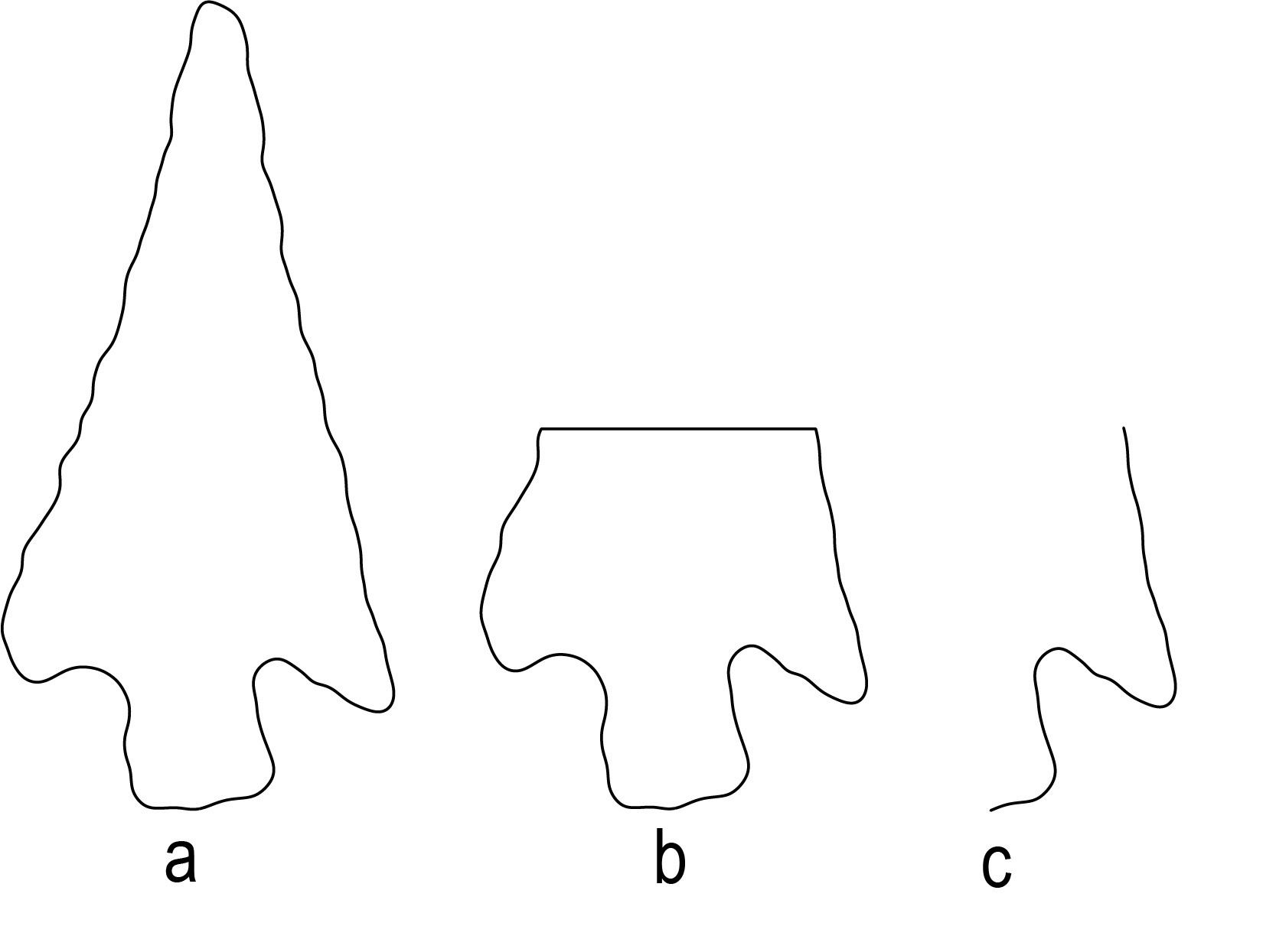
Figure 9: Demonstration of how a projectile point outline is reduced to one corner for geometric morphometric analysis.
Figure 10 shows the first two principal components, as well as the morphospace, which demonstrates the relationship between the principal components scores and the shape of the outlines. Side notch points and Parowan points are mostly separated from Rose Spring and Eastgate, although one point originally classified as Parowan appears to be misclassified. Rose Spring and Eastgate are, however, mostly overlapping.
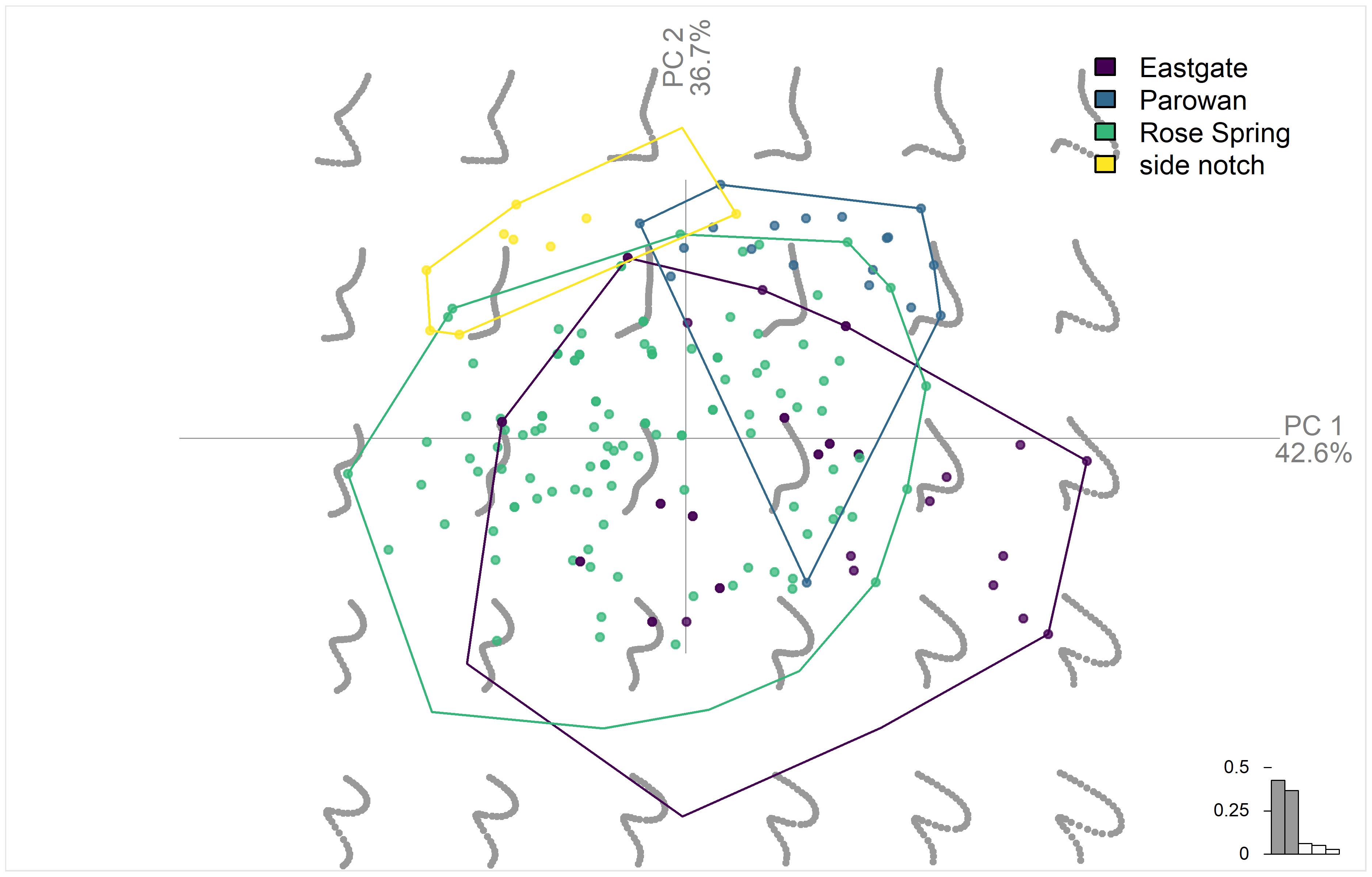
Figure 10: Principal components analysis of projectile points by type. The gray outlines show the morphospace, which demonstrates how the principal component axes affect the projectile point outlines. The bar chart in the bottom right shows the proportion of variation explained by each axis.
Using linear discriminant analysis (LDA) on the PCA results allows us to test how accurately the original typologies can be reproduced using this analysis. While true training and validation sets were not used in this small experiment, this provides a sense of how a GM approach compares to traditional methods. Table 4 shows the results of the predicted types using LDA and the original classification. The accuracy overall was 84% (n = 193). Each type had over 90% accuracy, except Eastgate which was 62%. The combination of Rose Spring and Eastgate into a Rosegate category would eliminate much of the error and increase the accuracy rate to 93%. The question remains, can Rose Spring and Eastgate points be reasonably separated, or should they be considered one type?
| Actual Type | Eastgate | Parowan | Rose Spring | side notch | accuracy |
|---|---|---|---|---|---|
| Eastgate | 28 | 1 | 16 | 0 | 62% |
| Parowan | 1 | 17 | 1 | 0 | 89% |
| Rose Spring | 4 | 5 | 108 | 2 | 91% |
| side notch | 0 | 0 | 1 | 9 | 90% |
Rose Spring and Eastgate points appear to lie along a continuous spectrum of morphological variability, but difficulty separating them may also be due to analyst error or to definitional error. The PCA plot does little to separate these two types, although the LDA analysis does a better job. Uniform manifold application and projection (UMAP) is a relatively recent algorithm for reducing dimensionality (McInnes et al. 2020). We use the algorithm as implemented through the “umap” package in R (Konopka 2020). The PCA results from the GPA analysis were used as the input for the UMAP algorithm and a K-means cluster analysis was used to create two groups. Figure 11 shows the results of this analysis. The K-means clearly only used one axis to separate the types. The group 2 points on the right-hand side would better fit group 1, but overall, this analysis produced a u-shaped distribution with some separation between the two groups. The original types, however, are not well separated.
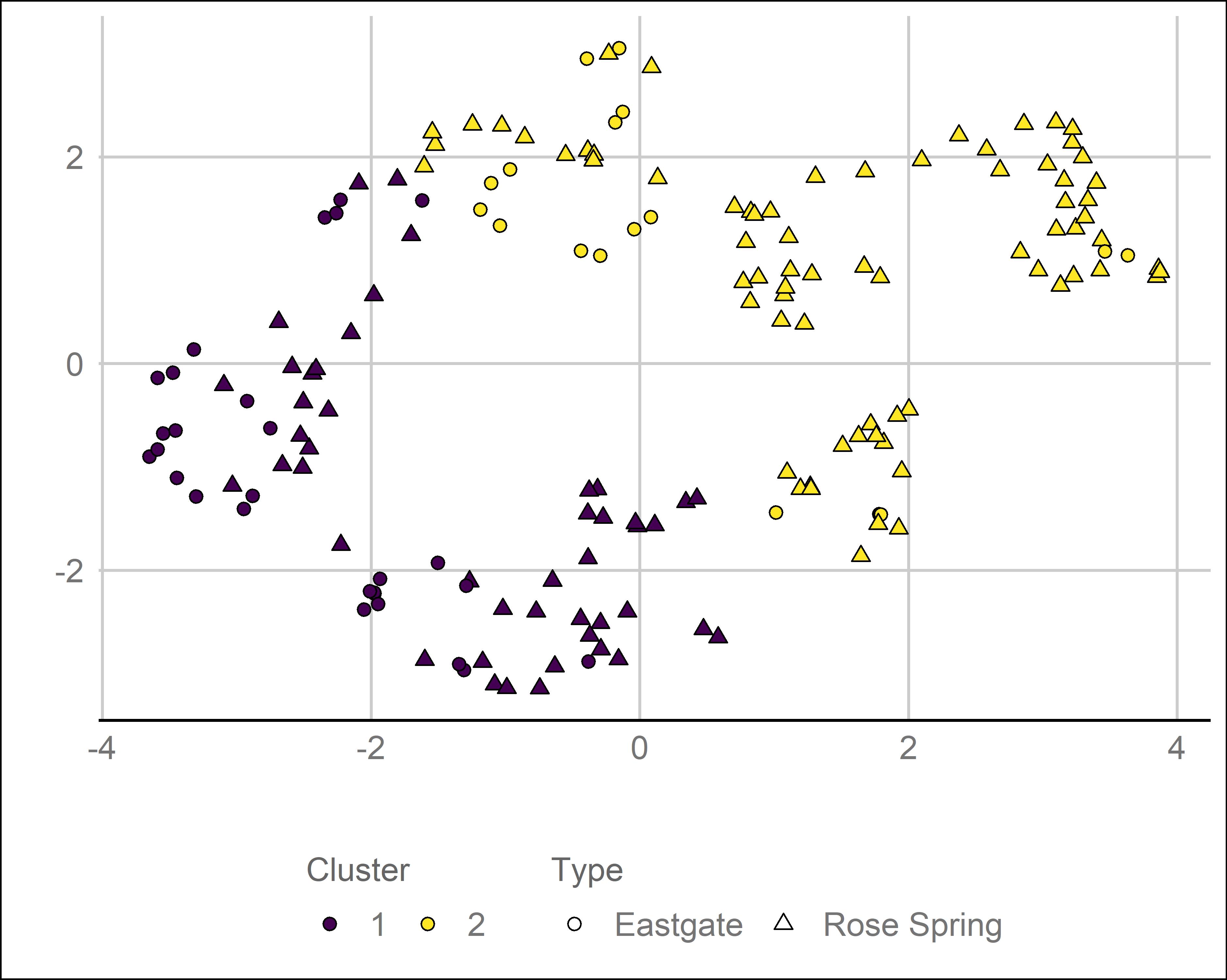
Figure 11: Biplot showing a uniform manifold approximation and projection of the principal components of a generalized Procrustes analysis, with the results grouped into two clusters using K-means cluster analysis. The original classification into Eastgate and Rose Spring are shown as circles or triangles.
This analysis suggests that Rose Spring and Eastgate cannot clearly be distinguished. Certain specimens are more clearly Eastgate or Rose Spring using the current definitions, but many points cannot be discriminated with reasonable certainty. Typologies are something we construct as necessary to make interpreting variation easier, but the difficulty of separating these types arguably supports the use of the combined Rosegate type, unless a particular research question requires a finer-grained distinction. If the types were to be redefined using a GM approach, then we would recommend a larger sample size and a more refined clustering approach.